• PDF
• Video

Table of Contents

Chapter 1 - The Budget Outlook

Chapter 2 - Economy, Revenues, and Demographics

Chapter 3 - Expenditure Projections

---

Executive Summary

Budget Situation Has Improved Sharply. The state’s economic recovery, prior budget cuts, and the additional, temporary taxes provided by Proposition 30 have combined to bring California to a promising moment: the possible end of a decade of acute state budget challenges. Our economic and budgetary forecast indicates that California’s leaders face a dramatically smaller budget problem in 2013–14 compared to recent years. Furthermore, assuming steady economic growth and restraint in augmenting current program funding levels, there is a strong possibility of multibillion–dollar operating surpluses within a few years.

The Budget Forecast

Projected $1.9 Billion Budget Problem to Be Addressed by June 2013. The 2012–13 budget assumed a year–end reserve of $948 million. Our forecast now projects the General Fund ending 2012–13 with a $943 million deficit, due to the net impact of (1) $625 million of lower revenues in 2011–12 and 2012–13 combined, (2) $2.7 billion in higher expenditures (including $1.8 billion in lower–than–budgeted savings related to the dissolution of redevelopment agencies), and (3) an assumed $1.4 billion positive adjustment in the 2010–11 ending budgetary fund balance. We also expect that the state faces a $936 million operating deficit under current policies in 2013–14. These estimates mean that the new Legislature and the Governor will need to address a $1.9 billion budget problem in order to pass a balanced budget by June 2013 for the next fiscal year.

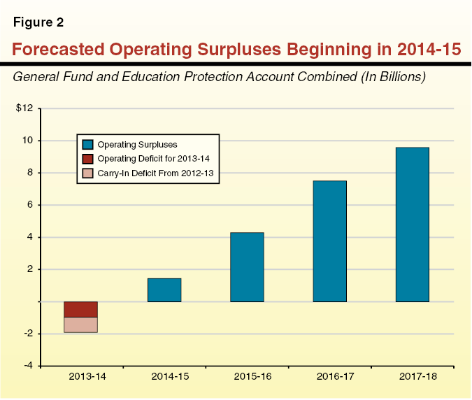
Surpluses Projected Over the Next Few Years. Based on current law and our economic forecast, expenditures are projected to grow less rapidly than revenues. Beyond 2013–14, we therefore project growing operating surpluses through 2017–18—the end of our forecast period. Our projections show that there could be an over $1 billion operating surplus in 2014–15, growing thereafter to an over $9 billion surplus in 2017–18. This outlook differs dramatically from the severe operating deficits we have forecast in November Fiscal Outlook reports over the past decade.

LAO Comments

Despite Positive Outlook, Caution Is Appropriate. Our multiyear budget forecast depends on a number of key economic, policy, and budgetary assumptions. For example, we assume steady growth in the economy and stock prices. We also assume—as the state’s recent economic forecasts have—that federal officials take actions to avoid the near–term economic problems associated with the so–called “fiscal cliff.” Consistent with state law, our forecast omits cost–of–living adjustments for most state departments, the courts, universities, and state employees. The forecast also assumes no annual transfers into a state reserve account provided by Proposition 58 (2004). Changes in these assumptions could dramatically lower—or even eliminate—our projected out–year operating surpluses.

Considering Future Budget Surpluses. If, however, a steady economic recovery continues and the Legislature and the Governor keep a tight rein on state spending in the next couple of years, there is a strong likelihood that the state will have budgetary surpluses in subsequent years. The state has many choices for what to do with these surpluses. We advise the state’s leaders to begin building the reserve envisioned by Proposition 58 (2004) as soon as possible. Beyond building a reserve, the state must develop strategies to address outstanding retirement liabilities—particularly for the teachers’ retirement system—and other liabilities. The state will also be able to selectively restore recent program cuts—particularly in Proposition 98 programs (based on steady projected growth in the minimum guarantee).

Chapter 1

The Budget Outlook

This publication summarizes our office’s independent projections for California’s economy, tax revenues, and expenditures from the state General Fund, as well as the Education Protection Account (EPA) created by Proposition 30. Our forecast is based on current state law and policies, as discussed in the nearby box.

The Budget Forecast

Projected $1.9 Billion Budget Problem Must Be Addressed by June 2013. The 2012–13 Budget Act assumed a year–end reserve of $948 million. As shown in Figure 1, assuming that no corrective budgetary actions are taken, we project that the state will close 2012–13 with a $943 million deficit. As discussed later, lower–than–expected savings related to the dissolution of redevelopment agencies (RDAs) and other budgetary erosions contribute to this shortfall. We also expect that the state faces an operating deficit in 2013–14—the difference between current–law revenues and expenditures in that fiscal year—of $936 million. These estimates mean that the new Legislature and the Governor will need to address a $1.9 billion budget problem in order to pass a balanced budget in June 2013 for the next fiscal year. This is a dramatically smaller budget problem than the state has faced in recent years.

Projected 2012–13 Deficit of $943 Million

Higher Spending and Lower Revenues Contribute to Deficit. The $1.9 billion deterioration in the 2012–13 budget situation is due to the impact of (1) $625 million of lower revenues in 2011–12 and 2012–13 combined, (2) $2.7 billion in higher expenditures, and (3) an assumed $1.4 billion positive adjustment in the 2010–11 ending budgetary fund balance. (The box on page 3 discusses the subject of revenue accruals—reportedly responsible for the fund balance adjustment—and other accounting issues related to the state budget.)

Revenue Estimates Down Somewhat From Budget Act Assumptions. The 2012–13 budget package assumed that Proposition 30 would pass—thereby temporarily levying additional personal income taxes (PITs) and sales and use taxes and depositing them to a new state fund, the EPA. Our forecast includes updated estimates concerning Proposition 30 tax receipts and the rest of the state’s revenues. It also adds increased corporation tax (CT) revenues based on voters’ approval of Proposition 39. For the General Fund and EPA combined, we currently project that 2011–12 revenues will be $348 million less than assumed in the 2012–13 budget package and that 2012–13 revenues will be $277 million less than assumed, for a total of $625 million less in revenues for these two fiscal years combined. The largest differences in this regard relate to the PIT and CT, as follows:

• Facebook Offsets Other Projected PIT Gains. Our updated estimate of revenues related to the initial public offering (IPO) of stock by Facebook, Inc., is lower than that assumed in the budget package—by $626 million spread across 2011–12 and 2012–13. On the other hand, our forecast of non–IPO PIT revenues is higher across these two fiscal years by $473 million. In total, PIT revenues in 2011–12 and 2012–13 are forecast to be $153 million below budget act assumptions. (Due to the state’s new revenue accrual policies related to Proposition 30, we note that the books will not be closed on 2011–12 revenues until at least a year from now.)

• Proposition 39 Revenues Offset Lower CT Estimates. Estimated CT revenues in 2011–12 were $605 million below the assumption in the budget act. In keeping with recent, very weak collection trends, we also forecast that CT revenues under prior tax law will be about $403 million lower than the budget act assumption in 2012–13. These declines, however, will be partially offset by the passage of Proposition 39, which changes the method by which some multistate businesses calculate their taxable income. We estimate that Proposition 39 will increase CT revenues by about $450 million in 2012–13. In total, therefore, our forecast of CT revenues in 2011–12 and 2012–13 combined is $558 million below the amount assumed in the 2012–13 budget act.

Significant 2012–13 Budget Actions at Risk. Our forecast projects $2.7 billion in higher expenditures will contribute to a year–end deficit in 2012–13. These include budgetary erosions associated with several actions adopted in the 2012–13 budget package, including the following:

• RDA Savings Will Be Much Less. As described further in Chapter 3, the budget package assumed about $3.2 billion in General Fund savings related to the dissolution of RDAs. We estimate, however, that the savings will total about $1.8 billion less than assumed in the budget.
• $400 Million of Cap–and–Trade General Fund Savings Unlikely to Materialize. The 2012–13 budget included savings associated with the state’s cap–and–trade program. Specifically, the budget package assumed that $500 million in revenues generated by the program’s auctions would offset costs traditionally supported by the General Fund. Consistent with our prior estimates, our forecast projects that only $100 million of such costs could be offset by the revenues, resulting in a $400 million budgetary erosion.
• Healthy Families Program (HFP) Costs. The 2012–13 budget package included a $183 million reduction to HFP. As explained in Chapter 3, our forecast assumes the reduction will not be put in place because it would violate a maintenance–of–effort requirement under the Patient Protection and Affordable Care Act, the federal health care reform law.
• Wildfire–Related Costs. The 2012–13 Budget Act included $92.8 million in General Fund support for emergency fire suppression activities. Due to heavy fire activity during the early part of 2012–13, CalFire has requested an additional $118 million in funding. While the federal government or local fire agencies will eventually reimburse the state for some of this funding, our forecast treats the entire amount as an increased cost because the amount of future reimbursement is unknown.

Relatively Small Budget Problem Forecasted for 2013–14

Many Factors Contribute to the 2013–14 Operating Deficit. The combination of recent spending reductions and temporary tax increases—plus improvement in the economy—has virtually eliminated the state’s “structural deficit.” Accordingly, we estimate that the state is poised to record a substantial operating surplus in 2012–13—which was necessary to eliminate most of the carry–in deficit related to prior years’ budgetary problems. In 2013–14, however, our forecast projects a $936 million operating deficit, assuming current law policies.

Many factors contribute to the small operating deficit we forecast in 2013–14. General Fund Proposition 98 payments, for example, grow by $1.8 billion. Also, actions to achieve savings in employee compensation—including furloughs and the Personal Leave Program—expire in June 2013, consistent with current labor agreements. Combined with scheduled pay increases and higher premium costs for state employees’ health care benefits, we project that employee compensation costs will increase by more than $750 million in 2013–14. We also project that General Fund debt–service costs related to infrastructure bonds will grow by $759 million in 2013–14. (These debt–service costs go up in 2013–14 primarily because the state structured its infrastructure bonds so that payments were lower in 2012–13. The state did this to accommodate the required, one–time repayment this year of a $2 billion loan from local governments, which the Legislature authorized in 2009 with its suspension of Proposition 1A [2004].)

The expiration of various one–time actions in the 2012–13 budget also contribute to the operating deficit, including about $419 million in higher expenditures for the judicial branch. We also assume that the state repays about $1.1 billion of loans to special funds, consistent with previous loan repayment schedules provided by the administration. (We note that the administration has substantial flexibility, in many cases, to delay such planned repayments.) Revenue growth of about $1.1 billion over 2012–13 partially offsets $3.7 billion in increased expenditures in our forecast.

Operating Surpluses Projected Over the Next Few Years

State “In the Black” After Years of Major Operating Deficits. Under current law, General Fund and EPA expenditures are projected to grow less rapidly than revenues, given our current economic forecast. Beyond 2013–14, we therefore project growing operating surpluses throughout the forecast period. As indicated in Figure 2, our forecast shows that there could be an over $1 billion operating surplus in 2014–15, growing thereafter to an over $9 billion surplus in 2017–18. A contributing factor to the surpluses beginning in 2016–17 is the end of the “triple flip,” the financing mechanism used for the 2004 economic recovery bonds (ERBs). (Specifically, the General Fund benefits—to the tune of about $1.6 billion per year—once the ERBs are retired, which will result in higher local funding for school districts and a related decrease in state funding requirements for schools.) This outlook of significant operating surpluses differs dramatically from the severe operating deficits we have forecast in November Fiscal Outlook documents over the past decade.

LAO Comments

Despite Positive Outlook,Caution Is Appropriate

Several Assumptions Key to Achieving Future Surpluses. Our multiyear budget forecast depends on a number of economic, policy, and budgetary assumptions that, if changed, could result in dramatically different outcomes. As discussed below, a variety of alternate scenarios would result in much smaller future operating surpluses or possibly operating deficits.

Revenue Forecast Assumes Steady Growth in the Economy and Stock Prices. Our forecast assumes steady economic growth, fueled in particular by recent encouraging data about the state’s housing market and income trends. In one alternative scenario we considered—assuming the economy underperforms and state revenues grow one–third slower than forecasted—80 percent of the surplus shown in Figure 2 for 2017–18 would be eliminated, and prior fiscal years would be much more likely to have an operating deficit. Our forecast also assumes steady growth in the stock market, which results in taxable capital gains. As we have pointed out many times over the years, these gains are notoriously volatile and hard to predict. They are a key reason why tax revenue forecasts can easily be a few billion dollars lower (or higher) than projected by us or the administration in any given fiscal year.

Federal Fiscal Policy Poses Risk to Revenue Forecast. As discussed in Chapter 2, the federal fiscal cliff poses a significant risk to our economic and revenue forecast. Specifically, if the Congress and the President are unable to resolve the fiscal cliff, the economy could enter recession beginning in 2013. We examined one possible recession scenario in which state revenues were about $11 billion lower than in our forecast for 2012–13 and 2013–14 combined. This scenario obviously would also delay any potential future operating surpluses.

Forecast Assumes No Transfers to the BSA. Proposition 58 (2004) generally requires 3 percent of estimated General Fund revenues to be transferred each year to the Budget Stabilization Account (BSA), the state’s rainy day fund. The state has made such transfers in the past, but the Governor has suspended the requirement annually since 2008–09 due to the state’s persistent budget problems. Our forecast assumes that no transfer will be made during the forecast period. As shown in Figure 3, however, a transfer of 3 percent of General Fund revenues to the BSA beginning in 2015–16 would reduce the operating surpluses by over $3 billion per year.

Forecast Assumes No COLAs or Inflation Adjustments. Consistent with state law and recent state policy, our forecast includes no cost–of–living adjustments (COLAs) or price increases over the forecast period, except when required under federal or state law. As shown in Figure 3, if we included COLAs and price increases for state operations (including the universities and the judicial branch) each year of the forecast, operating surpluses would be around $2.1 billion lower by 2017–18.

Forecast Does Not Account for Repayment of Many Obligations. Our forecast assumes that the state initiates no additional loans from special funds to the General Fund (except those already envisioned in the 2012–13 budget plan), and that these loans are repaid when scheduled or otherwise required—generally consistent with recent repayment schedules provided by the administration (and, in some cases, with repayment deadlines included in prior budget acts). As a result, in our forecast, the $4.3 billion loan balance currently owed to special funds by the General Fund is reduced to $3.1 billion by the end of 2013–14 and $1.2 billion by the end of our forecast period in 2017–18. The Governor, however, has stated his preference to pay down this and other elements of the so–called “wall of debt” within a few years. If the Legislature and the Governor seek to repay these obligations, surpluses could be lower in some years.

Revenue Volatility and Maintenance Factor. As discussed in our May 2012 report, Proposition 98 Maintenance Factor: An Analysis of the Governor’s Treatment, the maintenance factor approach used in building the 2012–13 budget can ratchet up Proposition 98 spending in certain situations. This ratcheting effect is most likely to occur in years with significant year–to–year increases in General Fund revenues. Because Proposition 98 appropriations in one year typically are used to calculate the minimum guarantee in the next year, a significant increase in the Proposition 98 minimum guarantee for one year also would likely increase the state’s obligations in future years. Although such ratcheting does not occur in our current forecast, this situation is possible over the forecast period, particularly given the inherent volatility of PIT revenues.

Proposition 30 Tax Increases Temporary. Proposition 30 increases the sales tax rate for all taxpayers through 2016 and PIT rates on upper–income taxpayers through 2018. In 2017–18, the last fiscal year of our forecast, we estimate that the higher PIT rates will raise about $5.6 billion in additional revenues. When those taxes expire beginning in 2018–19 (outside the time period considered in our forecast), ongoing surpluses could be several billion dollars lower.

Considering Future Budget Surpluses

As noted above, there are many ways that the future operating surpluses we now project could disappear or be reduced substantially. If, however, the state’s leaders choose to keep a tight rein on the budget over the next year and the economy avoids another recession over the next several years, they could experience the operating surpluses shown in Figure 2. During the 2013–2014 legislative session, lawmakers may want to begin considering how to use such potential surpluses. There are a variety of priorities for surplus funds, as described below.

Building a Reserve? As noted above, Proposition 58 generally requires that 3 percent of estimated General Fund revenues be deposited in the BSA, the state’s rainy day fund. Beginning in 2015–16, we project potential surpluses that would accommodate such a transfer. Within the next few years, we advise the Legislature and the Governor to begin building the reserve envisioned by Proposition 58, which could buy time to deal with the budgetary problem accompanying the next economic downturn. While our forecast does not assume such a downturn, one could easily materialize by 2018. For this reason, we favor BSA deposits as one priority for the use of available resources over the next few years.

Paying Down Budgetary Liabilities? As discussed above, our forecast assumes that special fund loans to the General Fund are paid back consistent with recent repayment schedules provided by the administration and that $1.2 billion of such loans remain outstanding by the end of 2017–18. The state could choose to pay down these loans faster. Paying down the loans faster would relieve the General Fund of some additional interest costs, allow special funds to either expand programs or reduce fees, and serve as a possible additional budget cushion for the General Fund during future recessions (since special fund balances available to be borrowed at that time could be larger). Other elements of the wall of debt (such as addressing the backlog of payments related to local government mandates) also could be funded from any surpluses that materialize. Still, other elements of the wall of debt could be retired with funds made available as part of the Proposition 98 minimum guarantee each year.

Addressing Retirement Liabilities? Unfunded liabilities of the state’s key pension systems—the California Public Employees’ Retirement System, the California State Teachers’ Retirement System (CalSTRS), and the University of California (UC) Retirement Plan—and the retiree health programs serving state government (including the California State University system) and UC represent funds not currently set aside to pay for benefits already earned by current and past public employees. While this year’s pension legislation reduces significantly the net employer cost of benefits that will be earned by future public employees, these unfunded liabilities must still be addressed. As such, one possible use for potential surpluses is paying down these significant liabilities, which total over $150 billion.

A key priority of the state in this regard probably should be a funding plan to address CalSTRS’ unfunded liabilities. Additional funding from the state, districts, and/or teachers of over $3 billion per year (and growing over time) likely will be required to keep CalSTRS solvent and retire its unfunded liabilities over the next several decades. Under a resolution approved by both houses of the Legislature this year, CalSTRS will submit several proposals in February 2013 for how to better fund the system in the future. Assisting UC in rebuilding the funding status of its pension system is another possible priority for surplus funds. Addressing these unfunded liabilities sooner likely would save state and local funds, compared to the costs of funding them down the road. This is because contributing funds to the pension systems sooner means that the systems can invest the funds and generate investment returns earlier than would otherwise be the case.

Selectively Restoring Cuts? The state has reduced spending in recent years in most areas, including health and social services programs, schools, universities and community colleges, the courts, and state administration. The state has also generally not provided COLAs or inflation adjustments for most of these programs. A key decision to consider for possible budget surpluses will be to what extent to use them to restore some of these cuts. (In Chapter 3 of this report, for example, we discuss potential priorities for the state in the use of increased Proposition 98 school funding over the next few years.)

Investing in Infrastructure? Another option for the use of potential surpluses would be investment in the state’s infrastructure. Our forecast, for example, assumes no additional bond authorizations for infrastructure even though several programs, such as K–12 and higher education, have exhausted most of their existing bond authority. Our forecast also does not include bond payment costs related to the $11 billion water bond now scheduled for the November 2014 statewide ballot. In our August 2011 report, A Ten–Year Perspective: California Infrastructure Spending, we noted various major infrastructure funding needs for the state, including those related to aging infrastructure and a growing backlog of deferred maintenance.

To effectively assess the enormous variety and complexity of the state’s infrastructure needs, the state needs a well–defined process for planning and financing projects. Unfortunately, the state does not have such a process. Particularly in the event that the state pursues a new infrastructure investment program in the coming years, a new approach to planning and financing it is needed, as we discussed in the August 2011 report.

Conclusion

The state’s economic recovery, prior budget cuts, and the temporary taxes provided by Proposition 30 have combined to bring California to a promising moment: the possible end of a decade of acute state budget challenges. If a steady economic recovery continues and the Legislature and the Governor keep a tight rein on state spending in the next couple of years, there is a strong likelihood that the state will have operating surpluses in subsequent years. The state has many choices for what to do with these surpluses. We advise the state’s leaders to begin to build the reserve envisioned by Proposition 58 as soon as possible. Beyond building a reserve, the state must develop strategies to address several substantial liabilities that will have to be paid—most notably, unfunded retirement liabilities and outstanding loans from the state’s special funds to the General Fund.

Chapter 2

Economy, Revenues, and Demographics

Economic Outlook

Figure 1 shows a summary of our forecast for both the U.S. and California economies through 2018. Figure 2 compares the near–term economic forecast with other recent California economic forecasts, including the Department of Finance’s (DOF) May Revision forecast (which was used as the basis for revenue assumptions in the 2012–13 Budget Act).

U.S. Economic Forecast Down, State Forecast Up From Budget Act Forecast. In general, our updated U.S. economic forecast is somewhat weaker than the forecast upon which the 2012–13 Budget Act was based. This is based on recent trends in the nation’s economy, including apparent hesitation by businesses to invest and hire due in part to uncertainty concerning future federal tax and fiscal policies. At the same time, we are somewhat more optimistic about the California economy than we were in prior months due to rising strength in the state’s depressed housing market, vehicle sales, and various employment trends. Nevertheless, as noted below, this remains a slow economic recovery by historical standards.

(We note that our economic forecast was developed prior to both the election and the date on which Hurricane Sandy struck New Jersey and New York. Sandy is likely to affect national economic data in the coming months. One possibility is that the storm’s effects will reduce U.S. gross domestic product [GDP] growth below our forecast by a few tenths of a percentage point in the fourth quarter of 2012, but add back about that amount to GDP in the following quarter due to reconstruction efforts.)

U.S. Economy

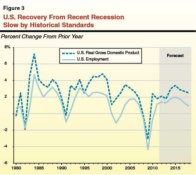
Slow Recovery From a Severe Economic Contraction. The 2007–2009 recession was the most severe economic contraction since the Great Depression. Moreover, as shown in Figure 3, the nation’s recovery from the recession has been slow by historical standards. Following the 1981–1982 recession, U.S. real GDP expanded at 3.5 percent or greater in each of the next four years, and the nation’s employment grew at 2.5 percent or greater in five of the six years during the 1984–1989 period. After the 1990–1991 recession, GDP grew by 3 percent to 5 percent in all but two years between 1992 and 2000, while employment grew by 2 percent to 3 percent annually through almost all of that period.

As shown in Figure 3, the current recovery—from the far more severe economic contraction of 2007–2009—is slower than the two recoveries described above in several respects. To date, GDP growth since the recession has been in the range of 2 percent per year, and we forecast that it will remain between 2 percent and 3 percent per year in all but one year between now and 2018. United States employment is forecast to grow at 2 percent or less each year through 2018.

Reasons for the Slow Recovery. Unlike other recent recessions, the 2007–2009 downturn was caused by an implosion of the nation’s financial sector and housing markets. This resulted in significant harm to banks’ balance sheets, as well as the balance sheets of households—particularly those that saw their net worth decline with the collapse of home values. Since the recession, financial institutions, households, and many businesses have been “deleveraging”—rebuilding their net worth and balance sheets step by painful step. Deleveraging requires saving, reducing consumption, and, in some cases, shedding liabilities through bankruptcies and renegotiation with creditors. Households and businesses are less capable of prodding the economy forward through spending, and financial institutions are less able to lend to facilitate such spending. These are some of the reasons why the U.S. economic recovery is so slow, relative to historical standards.

Federal Policy Important in the Forecast. The U.S. government borrowed significant amounts—including from international lenders—before, during, and after the recession to address the collapse of the financial sector, support some other economic sectors (such as the automotive industry and state and local governments), and provide economic stimulus. The Federal Reserve also has taken significant monetary policy actions intended to support the economy. As discussed later in this chapter, the U.S. government now faces major decisions about the future course of its fiscal and tax policies. These decisions have the potential to alter our economic forecast significantly over the next few years. In the worst case, federal decisions concerning the so–called “fiscal cliff” could plunge the U.S. economy into recession in 2013 and result in much weaker economic conditions in the near term than reflected in our forecast.

California Economy

California Also Recovering Slowly From the Recession. A similarly tepid recovery—compared to historical standards—is occurring in the California economy. The 2007–2009 recession was much more severe than recent downturns. Similar to the nation, personal income growth in California following the 2007–2009 recession has been much lower than after recent recessions. The rate of employment growth also has been slower. These trends are projected to continue in our forecast, although the recovery we are now projecting in the housing market is assumed to increase employment growth over the next four years, compared to what it would be otherwise.

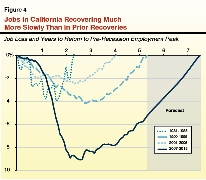
Figure 4 shows another way to look at the slowness of the current recovery in California. Covering the periods after the last four recessions, this figure shows how long it took California’s economy to return to the pre–recession peak level of jobs. After the 1981–1982 recession, it took over two years for the number of jobs in California to return to the pre–recession peak. After the 1990–1991 recession and the resulting cutbacks in the defense industry, it took over five years. After the 2001 recession and the bust of the “dot–com” bubble, it took four years. As shown in the figure, the total decline in jobs during and after the 2007–2009 recession—about 1.4 million jobs (9 percent of seasonally–adjusted employment)—was far greater than in the prior recessions shown. Moreover, the projected recovery period is much longer than for the prior recessions shown. Our forecast assumes that seasonally adjusted employment in California reaches its pre–recession peak in early 2015, or 7.5 years after its pre–recession peak in July 2007. (In 2015, California’s unemployment rate is projected to be around 8 percent—around 2 percentage points higher than it was in 2007—due in part to the state’s growing population over the period.)

Improvements in Job Market. Despite the slowness of this recovery, improvements in the state’s job market are evident. California now has regained 500,000 of the 1.4 million jobs it lost between July 2007 and February 2010, including a net gain of 262,000 jobs (1.9 percent) since September 2011. (This was faster than the national rate of employment growth—1.4 percent—over the same time period.) Due in part to some improvement in the housing sector, even California’s weakened construction industries now are adding jobs—up about 26,000 (4.7 percent) in the past year. Every category of construction jobs—except highway, street, and bridge construction—has contributed to these gains.

Manufacturing and Government Are Weak Job Sectors. While manufacturing employment has grown 1.5 percent for the U.S. as a whole over the past year, recent monthly jobs reports show that manufacturing jobs continue to decline in California—now down 11,000 jobs (0.9 percent) from one year ago. Moreover, while government employment has stabilized nationally, the combined number of federal, state, and local government jobs in California has declined—down 1.7 percent from one year ago. The bulk of the decrease is attributable to a drop of 35,000 jobs in local government educational services (a decline of 4 percent of jobs in this category). Manufacturing and government, therefore, are notable weak spots in an otherwise improving job situation in the state.

Housing Recovery Is Strengthening Somewhat

Recovery Has Been Slow. California’s housing market is well into its third year of recovery from the recent housing crisis, during which home prices declined substantially before hitting bottom in 2009. (The median existing single–family home price fell from $560,000 in 2007 to $275,000 in 2009.) The recovery has been anything but stable, marked instead by a series of false starts. Beginning in late 2009, for example, home prices in the state’s most populous areas—as shown in Figure 5—made solid gains for nine consecutive months before reversing trend throughout 2010 and 2011.

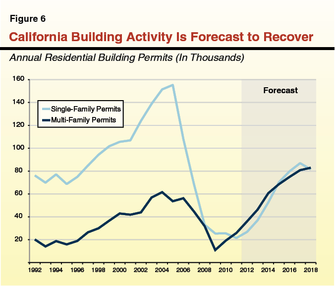
Construction activity also suffered during the housing crisis, coming to a near halt in 2009. As shown in Figure 6, single– and multi–family unit building permits declined from their combined peak of around 210,000 units annually in 2004 to just 36,000 units in 2009. Not surprisingly, construction–related jobs were one of the state’s most significantly weakened employment sectors.

Recent Housing Market Activity Stronger Than Previously Expected. A number of factors suggest that the demand for housing in California has picked up significantly from last year. Home prices in Los Angeles, San Diego, and San Francisco increased for the eighth consecutive month in August. Prices also have increased lately in the area’s most affected by the housing crisis: the Central Valley and the Inland Empire. In addition, monthly rents have increased throughout the coastal regions of the state, with some areas posting double–digit annual increases. Not only do large annual rent increases act as a signal to developers to build more units, they can also indirectly affect the market for single–family homes. Specifically, as the cost to rent increases more quickly than the cost to own, many current renters may find that is has become comparably more affordable to purchase a home, further bolstering the modest housing recovery. Finally, a recent jump in the number of building permits—an indicator of future housing activity—suggests that housing development may already be responding to recent demand indicators.

Current Forecast Projects Recent Strength to Continue. We view the trends discussed above as potentially more sustainable than those associated with earlier signs of housing strength, which proved largely illusory. Accordingly, we now forecast housing activity in the state to build upon current trends and stabilize in the final years of our forecast at approximately 160,000 new units annually, as shown in Figure 6. We forecast growth in both single– and multi–family unit building activity. Although our forecast level of building permits is much lower than during the housing boom of the mid–2000s, it remains a substantive upward adjustment in this forecast compared to our previous projections. This strength carries over to our forecast for assessed property values and property taxes, which is discussed in the nearby box.

Considerable Uncertainty Due to Difficulties in Forecasting Housing Trends. Forecasting housing activity is difficult because housing is influenced by complex and often unpredictable economic relationships. These include broad indicators like income and employment growth; real estate metrics like credit availability, mortgage rates, affordability, and prices (which may be subject to speculation); as well as behavioral markers like household formation and consumer confidence. In addition, the most recent data used in most economists’ forecast models—including our own—are from two atypical periods: the housing boom of the mid–2000s and the ensuing crisis of the past few years. Forecasting future housing activity relies heavily, therefore, on judgment and is prone to significant upward and downward variation. Because of the importance of the housing market to the state’s economy, housing activity below the levels in our forecast would in turn influence other key economic variables. For example, should building permits peak at 120,000 units annually (somewhat below our expectation of 160,000 units), the state’s sales tax base could grow about one–half of a percentage point slower each year through 2017–18 than our current forecast assumes. Construction employment and, therefore, income taxes also would be affected.

Federal Policy

As noted in Chapter 1, the fiscal cliff is a key uncertainty in this forecast. All economic and tax forecasts are based on assumptions about future federal tax, spending, and regulatory policies. Similar to recent forecasts from our office, the administration, and many economists, this forecast assumes that the President and the Congress agree to actions in the coming weeks to delay or eliminate the tax increases and spending cuts of the fiscal cliff in the near term. We believe this is the most likely type of outcome.

Tax Policy Issues Are the Key Short–Term Risk for the State Budget. We believe that the most significant fiscal cliff issues affecting the state budget in the near term are the tax policy decisions facing the President and the Congress. Under current federal law, many federal taxes are scheduled to rise in 2013—potentially increasing tax liabilities of about 90 percent of the population. The following tax increases (or end to temporary tax reductions) are scheduled to occur as part of the fiscal cliff:

• The end of the “Bush tax cuts” (which were extended during the Obama administration), resulting in increased federal income tax rates for the vast majority of all taxpayers and a variety of other tax changes. Among the tax changes are higher capital gains and dividend tax rates for many taxpayers.
• The expiration of the 2 percentage point reduction in Social Security payroll taxes in effect for the last two years—increasing the taxes of about 120 million households.
• Increased applicability of the federal alternative minimum tax (AMT)—potentially affecting tens of millions of taxpayers nationwide—in the coming months due to the fact that there has not yet been an AMT “patch” passed for 2012. (Taxpayers in states with relatively high state or local taxes—such as New York, New Jersey, and California—may be the most likely to be affected if there is no AMT patch.)
• An additional 0.9 percent tax on higher–income taxpayers’ earnings and a new 3.8 percent investment surtax on higher–income taxpayers’ capital gains, dividend, and interest income over certain thresholds, among other tax changes included in the Patient Protection and Affordable Care Act (the federal health care reform law).
• The expiration of several expanded tax credits for low–income households adopted during the Obama administration, such as the expansion of the earned income tax credit adopted as part of the 2009 federal stimulus package.
• The expiration of various other short–term tax provisions that Congress regularly extends (known as “extenders”), such as the adoption credit, the deduction for qualified education expenses, and the research and experimentation business tax credit.
• The end to the temporary “bonus depreciation” business tax provision for new investments, which has allowed companies to expense more costs of qualified machinery and equipment, rather than claiming deductions for depreciation over time.
• A resumption of pre–2000 federal estate tax rates and exemption amounts, which could result in the number of estates subject to this tax increasing by more than ten times.

In addition to the tax increases, a broad array of domestic and defense–related spending cuts—some of which are to be implemented via the federal government’s “sequestration” process—are scheduled to begin in 2013. (These would impose on many programs an across–the–board spending cut—generally between 8 percent and 10 percent—but would not directly affect most of the major federal funding streams that flow through the state treasury.) Extended emergency unemployment insurance (UI) benefits also are scheduled to expire, which would shorten significantly the amount of time that some unemployed workers are eligible for benefits.

Forecast Assumes That Washington Avoids the Fiscal Cliff. As noted above, our economic and budgetary forecast assumes that the President and the Congress adopt measures in the next few weeks to delay or eliminate virtually all of the near–term tax increases and spending cuts of the fiscal cliff. Instead, we assume that federal officials eventually reach agreements that involve spending cuts and tax increases, phased in over many years, to address the federal government’s serious long–term budgetary challenges. Our forecast also assumes that the necessary increase in the federal debt ceiling in 2013 causes little or no disruption to the economy, including consumer confidence.

Recession Likely if Federal Leaders Are Deadlocked. If the President and the Congress cannot come to an agreement and the fiscal cliff tax increases go into effect (particularly when combined with the domestic and defense federal spending cuts in the current sequestration law), the U.S. economy likely would fall into recession in 2013. This in turn would cause the California economy to perform considerably weaker than we assume in our forecast and reduce state revenues substantially in the near term. In an alternative simulation in which we assumed a 0.6 percent contraction of real U.S. GDP in 2013—rather than the 1.8 percent increase in our forecast—state revenues in 2012–13 and 2013–14 combined were about $11 billion lower than indicated in our forecast. (For the state’s General Fund expenditures, such a revenue reduction would be accompanied by a lower Proposition 98 minimum guarantee and higher spending requirements under current law for various health and social services programs.) The bulk of the assumed drop in GDP in this alternative recession scenario results from the expiration of the Bush tax cuts and the payroll tax cut. Spending cuts, the end of the bonus depreciation policy, and the expiration of emergency UI benefits each are responsible for a smaller part of this hypothetical near–term economic contraction.

Policy Uncertainty Hindering U.S. and Global Economic Growth. The perception of political paralysis concerning economic policy in the U.S., Europe, and China has constrained global economic growth in recent months. These issues contribute to our weaker projections for near–term U.S. economic growth. Exports and business fixed investment had—until recently—been key drivers of the current global economic recovery, but U.S. export growth has slowed. Exports to China are growing at only 2.2 percent on a year–over–year basis, while exports to Europe have been down recently—both figures related to the weakened economies of those important trading partners. Our forecast assumes that business investments in structures, equipment, and software are now growing more slowly than before—a trend that could affect California’s technology and service sectors in the coming months. In general, uncertainty about federal tax and spending policy inhibits risk taking and causes businesses and consumers to be more cautious in their spending and investment decisions. While there are “downside” risks due to the fiscal cliff, we note as well that there are “upside” risks to our economic forecast. If, for example, there is a speedy agreement concerning these federal issues, this could be looked upon favorably by consumers and businesses, thereby encouraging them to spend, invest, and hire even more in the short term than we are projecting.

The Demographic Outlook

Domestic and International Migration Expected to Climb. A summary of the key findings of our California population forecast is shown in Figure 7. Over the next several years, we project steady overall growth in the state’s population of about 1 percent per year. Migration into California—from other states and countries—declines during periods of relative economic weakness here. As Figure 7 shows, we estimate that the state has recently experienced significant declines in domestic migration (that is, many more people have left California for other states than have come from other states). Our forecast projects that these trends are turning around, and total net migration (domestic and international) will be positive over the forecast period. The state’s population—now just over 38 million—is projected to surpass 40 million in 2017.

Our forecast assumes continued declines in both birth rates and death rates. Specifically, women are waiting until later to have children and are having fewer children, on average, than in the past. This trend is largely responsible for a projected small decline in the state’s school–age and college–age populations between the 2010 and 2020 censuses. We forecast that there will be 6.7 million Californians age 5–17 in 2020 (down 1.4 percent from 2010) and 3.8 million who are age 18–24 (down 2.8 percent from 2010). In addition, Californians are living longer and this—coupled with the aging of the massive post–World War II “baby boom” generation—is resulting in large increases in the elderly population. We forecast that there will be 6.5 million Californians age 65 and over in 2020 (up 51 percent from 2010).

California’s Racial and Ethnic Makeup Continues to Change. In 1980, about 67 percent of Californians were non–Hispanic whites, and about 19 percent were Hispanic. By 2010, the census indicated that 40 percent of the state’s population consisted of non–Hispanic whites, and Hispanics made up 38 percent of the population. During the same time period, Asian Americans climbed from 5 percent to 13 percent of the population. African Americans made up 6 percent of the population in 2010, down from 7.5 percent in 1980.

In the next few years, the number of Hispanic Californians should surpass the number of non–Hispanic white residents. In 2020, we project that Hispanics will comprise 39 percent of the state’s population, followed by non–Hispanic whites (37 percent), Asian Americans (14 percent), African Americans (6 percent), and other racial and ethnic groups (4 percent).

Revenue Outlook

Figure 8 shows our multiyear forecast of General Fund and Education Protection Account (EPA) revenues, including revenues resulting from the two tax–related measures that voters approved at the statewide election on November 6, 2012. These two measures are Proposition 30 (which increases personal income tax [PIT] rates for higher–income Californians through 2018 and raises the sales and use tax [SUT] rates by 0.25 percentage points for four years beginning in 2013) and Proposition 39 (which institutes a new corporation tax [CT] apportionment policy that will result in some businesses paying more in taxes).

Figure 9 compares our revenue forecast for 2011–12 and 2012–13 to other recent forecasts. (Additional figures comparing this forecast with other recent forecasts are available on our website.)

Personal Income Tax

Little Net Change in Budget Act Revenue Assumptions. Before considering the passage of Proposition 30, which will generate some revenue that the state plans to attribute—or “accrue”—to 2011–12, PIT revenues for the prior fiscal year currently are estimated to have been $50.4 billion. After including our current projections for Proposition 30 collections, we now estimate that 2011–12 General Fund and EPA PIT revenues will total $53.2 billion, $255 million above the level assumed in the 2012–13 budget package. In 2012–13, we project PIT revenues to reach $59.9 billion, $408 million below the level assumed in the 2012–13 budget package. Therefore, for the two fiscal years combined, our PIT forecast is $153 million below the level assumed in the budget plan. For such a large, volatile revenue source, this is a minor forecasting difference.

The over $6.6 billion of year–to–year growth between 2011–12 and 2012–13 is due to (1) a full fiscal year of increased revenue under Proposition 30, (2) assumed growth in the economy and stock market, and (3) 2012–13 revenues related to Facebook, Inc.’s initial public offering (IPO) of stock.

About 6 Percent Annual Growth in PIT Revenues Forecast. For 2013–14, we forecast General Fund and EPA PIT revenue to grow to $61.7 billion, with steady growth thereafter, reaching $79.8 billion in 2017–18. Between 2012–13 and 2017–18, we forecast average annual growth in PIT collections of 5.9 percent.

Strengthening Job Market Helps PIT Revenues. The PIT is the state’s largest General Fund revenue source and grows over time largely in line with the main component of taxable personal income: the wages and salaries of Californians. The most recent data for 2010 indicate that wages and salaries made up 73 percent of California resident tax filers’ adjusted gross income (AGI) and accounted for 63 percent of PIT revenue. Accordingly, the strength of trends in the state’s job market plays a major role in the PIT’s overall growth rate.

Consistent with the decline in employment in the state during 2008 and 2009 (illustrated earlier in this chapter in Figure 4), resident tax filers saw their wage and salary income drop from $716 billion in 2008 to $679 billion in 2009 (down 5.2 percent). In 2010, wages and salaries grew to $697 billion (up 2.7 percent). The Franchise Tax Board (FTB) will provide us with our first solid data on 2011 wages later this month, but based on 2011 and 2012 PIT collections, economic data, and our forecasting estimates, we currently assume that wages and salaries grew to about $730 billion (up 4.6 percent) in 2011. The significantly greater increase in wages and salaries in 2011 was driven by the start of the state’s job recovery in that year.

Furthermore, based on data received to date for 2012, we assume that wages and salaries will grow to $774 billion (up 6 percent) in 2012. As 2012 job growth in the state is faster than that in 2011, so is the growth in overall taxable wages. (A small portion of this 2012 gain represents taxable income that higher–income Californians, in particular, are projected to accelerate—that is, choose to receive early—in order to benefit from lower federal tax rates in current law before the scheduled fiscal cliff tax increases.)

Our forecast model assumes that California resident tax filers’ wage and salary income surpasses $1 trillion for the first time in 2017. Between 2012 and 2018, we assume that wages and salaries for all resident California taxpayers grow at an average annual rate of about 5 percent—similar to the growth rate in recent decades. Employment growth, inflation, and changes in labor productivity contribute to rising wages and salaries throughout the economy.

Capital Gains Drive PIT Volatility. Net capital gains made up only 6 percent of AGI in 2010 and 3 percent in 2009, but this relatively small part of overall income is the most difficult element of the PIT to project. Net capital gains—the difference between capital gains and capital losses reported on tax returns—represent net investment gains from sales of assets such as stocks, bonds, and real estate. Data suggest that the single greatest driver of capital gains trends is the direction of the stock market. All economic models must make assumptions about stock market trends, as does ours. Nevertheless, in any given time period, the stock market can move up or down in ways that are both wildly volatile and inconsistent with trends elsewhere in the economy. As such, capital gains forecasts are subject to a wide band of uncertainty.

While capital gains made up 6 percent of AGI in California in 2010, personal income taxes paid on these capital gains totaled 10.5 percent of overall PIT paid that year, according to FTB estimates. The typical dollar of capital gains is taxed at a higher rate than the typical dollar of wage and salary income. In 2010, 15 percent of total AGI was reported on tax returns that had AGIs of $1 million or greater. By contrast, over 75 percent of capital gains were reported on returns with taxable income of $1 million or greater. Returns with $10 million or more of taxable income had 46 percent of all capital gains.

Net capital gains reported by resident tax filers climbed as high as $120 billion in 2000 (equal to 10.6 percent of personal income) and $132 billion in 2007 (8.4 percent of personal income), as shown in Figure 10. Such increases were driven by “asset bubbles” in the stock market and/or the real estate market. Net capital gains fell to $29 billion in 2009 (1.9 percent of personal income) before rising, along with the recovery in the stock market, to $55 billion in 2010 (3.5 percent of personal income). While the stock market has grown fairly well during much of the time since then, we assume that net capital gains remained fairly flat in 2011, given the substantial losses that investors experienced during the recession (which “offset” the gains that they report). Figure 10 shows our forecast for net capital gains, including gains assumed to be accelerated from 2013 to 2012 due to the lower federal tax rates currently in federal law prior to the fiscal cliff.

Volatility Likely to Increase Due to Proposition 30. As described above, the volatility in the stock market will contribute to PIT revenues being lower or higher than reflected in our forecast in each fiscal year. Because Proposition 30 increases the dependence of the state budget on revenues paid by higher–income taxpayers, who receive most capital gains, it is likely to increase the volatility of revenues through 2018. Also, as we noted in the November 2012 Voter Information Guide, uncertainty concerning the responses of high–income taxpayers to Proposition 30’s income tax increases may make these new revenues particularly difficult to estimate. These issues can easily cause actual PIT revenues to be a few billion dollars lower or higher than projections in any given year.

Facebook Stock Slump Offsets Other Projected PIT Gains. The May 2012 IPO of stock by Facebook, Inc. was plagued by technical mishaps and other concerns, and the company’s stock prices lagged far below budget act assumptions in the ensuing months. This forecast assumes the state’s IPO–related General Fund revenues total $1.25 billion in 2011–12 and 2012–13 combined—down from the $1.9 billion assumption in the budget act. While taxpayer confidentiality laws mean that there never will be a precise estimate of this total, sharp increases in daily state tax collections following both the IPO and the settlement of restricted stock units (RSUs) by Facebook employees—as well as Facebook’s public filings—suggest that most of this amount already has been collected by the state. Other revenues are likely to be collected in conjunction with future RSU settlement activity, estimated tax payments, final returns, and tax extension payments. We also assume that 2013–14 General Fund revenues related to the IPO will be $310 million.

Our forecast of 2011–12 and 2012–13 PIT revenues not related to the IPO are higher than those assumed in the budget act and in our office’s May Revision revenue forecast. Compared to the budget act PIT assumptions, our projected increase in non–IPO PIT revenues ($473 million for the two fiscal years combined) mostly offsets our projected decrease in IPO–related PIT revenues ($626 million).

Given that future IPO–related tax collections will simply be “lumped in” with other PIT collections, this likely will be the last time that we are able to estimate specific, discrete numbers for Facebook IPO–related revenues. In the future, IPO–related RSU settlements and options also will be lumped in with other official economic data, such as personal income data released by the federal government.

Sales and Use Tax

Estimated SUT revenue totaled $18.9 billion in 2011–12, $62 million lower than the amount assumed in the 2012–13 budget. In 2012–13, we expect SUT receipts to increase 10.5 percent to $20.8 billion ($234 million above the 2012–13 budget assumption). The growth in 2012–13 is the result of (1) the temporary one–quarter cent SUT increase under Proposition 30 and (2) growth in underlying taxable sales. (Proposition 30 increases the statewide SUT for four calendar years—2013 through 2016—meaning that it affects half of fiscal year 2012–13 and all of 2013–14.) For 2013–14, we forecast SUT revenue to increase 9 percent to $22.7 billion. The SUT revenues then grow more modestly—at an annual rate of 4.6 percent over the final four years of our forecast. The slower growth in SUT receipts in the out–years also reflects the expiration of the temporary rate increase.

Trends in Taxable Sales. The main determinant of SUT receipts is taxable sales—the amount spent by individuals and businesses on goods that are subject to the SUT. Significant components of General Fund taxable sales include vehicle sales (9 percent of taxable sales), construction materials used to build residential and commercial properties (6 percent), and consumer spending on dining (12 percent), electronics (3 percent), and furniture (2 percent). About two–thirds of taxable sales are consumer spending, whereas the remainder is business–to–business transactions where the purchasing business is the final user of the product. (Business purchases that become part of a final product are not subject to the sales tax.)

Consumer and business spending on taxable items declined 14 percent in 2009, as income levels fell, savings rates climbed, and economic uncertainty shattered consumer confidence. As shown in Figure 11, however, taxable activity—measured by taxable sales as a share of personal income—has recovered strongly, in part because consumers and businesses are now making large purchases that were postponed during the recession. We expect the recent increase in taxable sales as a share of personal income to moderate throughout the rest of our forecast as businesses and consumers normalize spending patterns.

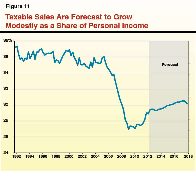
Optimism Concerning New Vehicle Sales and Housing Activity. Our current forecast of taxable sales is slightly stronger than our most recent forecast, developed for the May Revision. This improvement reflects a more optimistic outlook for new vehicle sales and housing activity over the next five years, an outlook supported by recent economic reports. For example, new vehicle sales increased 35 percent in the third quarter of 2012 (from levels a year earlier) and the S&P/Case–Shiller Index of housing prices has seen consistent gains throughout 2012. Increasing home prices and monthly rents tends to spur construction activity as developers build additional units to meet rising housing demand. We expect these trends to continue, especially given the improved outlook that many consumers have about the economy. In October, for example, the Reuters/University of Michigan Consumer Sentiment Index rose to 82.6 points, its highest level since the recession began.

Corporation Tax

Estimated CT revenue totaled $7.6 billion in 2011–12, $605 million below the 2012–13 budget act assumption. We forecast that General Fund CT revenue will be $8.5 billion in 2012–13, $47 million above the budget assumption. This 2012–13 forecast—unlike the budget act forecast—includes additional revenue projected to be raised under the new mandatory single sales factor provisions of Proposition 39. If Proposition 39 had not passed, our 2012–13 CT projection would have been $403 million short of the budget act forecast. Below, we discuss possible reasons for this weakness in baseline CT revenues. Our forecast further reflects the assumption that CT revenue will grow from $8.5 billion in 2012–13 to $10 billion in 2017–18—an average annual growth rate of 3.2 percent during that time period. (About one–third of this growth is attributable solely to Proposition 39, given that the half–year revenue effect in 2012–13 grows to a full–year revenue effect in 2013–14 and beyond. If Proposition 39 had not passed, the growth rate would be a much weaker 2 percent per year.)

National Corporate Profit Data Was Revised Downward. The vast majority of California CT revenue is paid by multistate and multinational corporations that apportion (allocate) a share of their profits to California. The 2012–13 Budget Act was premised on an assumption that national corporate profits had grown from $1.4 trillion in 2009 to $1.8 trillion in 2010—a 32 percent increase. (Our office’s May Revision estimates were based on a similar forecast for 2010.) In August, the federal Bureau of Economic Analysis revised the 2010 national corporate profits figure down to $1.7 trillion—a 27 percent increase over revised 2009 figures. This data revision results in our current forecast for national profits being about $100 billion less in each year compared to the economic forecast upon which the budget act was based. (The revision also may help explain part of the reason why CT revenues have fallen so far short of state projections over the past year.)

Flat Corporate Profits Projected. Similar to our recent forecasts, we assume weaker national profit growth in later years. We now assume profits remain relatively flat over the forecast period. Recent profit gains likely were the result of the “bounce back” after the recession and cost cutting, including flexibility in labor costs. Some corporations also have benefited from low borrowing costs, which, like labor costs, are likely to rise as the economy gains strength.

Recent Tax Policy Changes Have Reduced CT Revenues. As we described in our February 2012 publication, The 2012–13 Budget: Economic and Revenue Update, the state has undertaken a variety of corporate tax policy actions in recent years. Collectively, the effect of several of the state’s policy actions was to accelerate CT collections from 2011 and beyond back to 2007–08, 2008–09, and 2009–10 in order to help the state’s budget situation during the recession. These policy changes appear now to be reducing CT revenues, as intended. The policy actions included the suspension, for 2008 through 2011, of larger businesses’ use of net operating loss deductions. In addition to these accelerations of CT revenue, the state also changed corporate tax policies in order to reduce taxes for some businesses—such as the adoption of the elective single sales factor method of profit apportionment and allowing the transfer of credits among companies treated as part of a single business group for tax purposes. In total, the major changes to CT policies likely are reducing General Fund revenues by over $2 billion per year, as of 2012.

Proposition 39 Increases CT Revenues. Proposition 39—which will affect corporations’ 2013 and subsequent tax returns—partially reverses the recent policy trend of reducing CT revenues. Proposition 39 eliminates the elective single sales factor policy now in effect and replaces it with a requirement for most multistate corporations to apportion profits to California based on the single sales factor method. This will result in some corporations paying higher taxes resulting in projected half–year revenues of $450 million in 2012–13 and an estimated $1 billion per year thereafter. For the five fiscal years 2013–14 through 2017–18, however, the proposition dedicates half of the revenues—up to $550 million annually—for clean energy projects. (This latter portion of Proposition 39 revenues is not included in Proposition 98 revenue calculations in our forecast.)

Recent Policy Changes Complicate Forecasting Significantly. Our revenue forecasting models use statistical tools to identify relationships between economic and tax data in the past and then forecast how those relationships will play out in the future. These tools work best in a stable tax policy environment. Recent weakness in CT revenues—potentially related to recent policy changes—has been so significant that our confidence in standard forecasting models has declined. As with the PIT, additional data on recent years’ CT collections will be available from FTB later this month. It probably will take several more years—assuming a stable policy environment in the future—in order to recalibrate and improve our forecasting models in light of the new policies in place. The CT has always been a difficult tax to forecast, with many factors influencing the amount of taxes businesses owe the state in any given year. It will remain much more difficult to forecast than usual for a few more years.

Estate Tax

Federal Actions Necessary to Resume State Tax Are Very Unlikely to Occur. In 2001, as a part of the tax reductions enacted during the Bush administration, the federal government adopted reductions over several years to its estate tax and eliminated a tax code provision known specifically in state and federal law as the “Credit for State Death Taxes.” The state credit was eliminated entirely for estates of those dying after December 31, 2004. In 2010, the Congress and President Obama agreed to extend the temporary 2001 estate tax legislation—including elimination of the state death tax credit—until the end of 2012. Under current federal law, therefore, the pre–2001 estate tax regime will resume at the beginning of 2013 (part of the fiscal cliff), including the state credit.

Most observers believe that, no matter what Congress does to the estate tax in the coming months, there will no longer be a credit for state–level estate taxes. Our forecast assumes that this consensus is correct. Pursuant to Proposition 6 (1982), the state may only collect estate taxes equal to the Credit for State Death Taxes in federal law. Accordingly, our forecast assumes that the state receives no estate taxes related to deaths that occur in the future. We again advise the Legislature to assume no such revenues unless there is a clear indication from the Congress that such a tax credit will be adopted. If our assumption is wrong, the amount of funds the state will collect will depend on the details of whatever estate tax legislation is enacted at the federal level. (These additional revenues, if they were to be received, also would increase the state’s Proposition 98 minimum guarantee.)

Transfers

General Fund’s Budgetary Loans From Special Funds Now Total $4.3 Billion. The state has lent balances of its special funds to the General Fund in order to address budget shortfalls over the last decade. When the General Fund is directed to repay such a loan, this is booked as a transfer out of (a “negative” transfer from) the General Fund—for the repayment of principal. (The state also incurs expenditures to pay interest on these loans—generally linked to a measure of what the special fund otherwise would have earned in interest in the state investment pool.) In effect, such transfers out reduce overall General Fund revenues in the state’s budgetary accounting system. Figure 8—earlier in this chapter—shows projected net transfers and loans in each fiscal year, including special fund loan repayments.

In July 2012, DOF reported that the General Fund owed $3.6 billion in loan principal repayments to special funds. Given another $713 million of new loans authorized in the 2012–13 budget plan, the General Fund now has $4.3 billion of outstanding budgetary loans from the state’s special funds. (These loans were one of the components of the Governor’s “wall of debt” listing.)

Forecast Assumes Loans Repaid Pursuant to Schedule Provided by Administration. The July DOF report included anticipated repayment dates for many, but not all, outstanding General Fund loans (which sometimes were based on loan repayment deadlines in prior budget acts). Our forecast generally assumes that loans are repaid on the dates that DOF listed (as modified by the 2012–13 budget package in some cases), unless we identified a specific reason why a special fund might need an earlier repayment. For example, Figure 12 shows the special fund loans assumed in our forecast to be repaid by the end of 2013–14. In our forecast, the $4.3 billion balance described above is reduced to $3.1 billion by the end of 2013–14 and $1.2 billion by the end of 2017–18. (The $1.2 billion of remaining loans is assumed to be paid after 2017–18 in our forecast, since the DOF report includes no specific repayment dates for these.) Accordingly, to achieve the Governor’s stated goal of paying down entirely this element of the wall of debt within the next few years, additional loan repayments—above the level included in our forecast—would be required.

Legislature Has Considerable Flexibility Concerning Loans Under Recent Case Law. The increased prevalence of special fund budgetary loans to the General Fund has been the subject of recent litigation. In two 2011 appellate court cases—concerning loans to the General Fund from the Contingent Fund of the Medical Board of California and the Beverage Container Recycling Fund—judges rejected claims from litigants that these particular loans compromised special fund purposes or transformed regulatory processing fees into taxes (which arguably might have required a two–thirds vote of the Legislature). In one of the cases, the court stated that allowing the special fund loans to remain in place was a “reasonable and practical result that gives the state flexibility to balance its budget in a manner that does not stymie beneficial regulation.” We read these decisions to give the Legislature considerable, continuing flexibility related to special fund budgetary loans. At the same time, the decisions suggest that the Legislature has some measure of responsibility to ensure that special fund programs adequately meet the responsibilities for which the funds’ revenues were levied in the first place.

In this chapter, we discuss our expenditure estimates for 2011–12 and 2012–13, as well as our projections for 2013–14 through 2017–18—both for the General Fund and the Education Protection Account (EPA) created by Proposition 30. Figure 1 shows our projections of General Fund expenditures for major programs. Below, we discuss estimated General Fund spending for 2012–13 and expenditure trends in the forecast period. Thereafter, we discuss our expenditure projections for individual program areas.

2012–13 Outlook

We estimate that General Fund expenditures in 2012–13 will total roughly $94 billion, about 7.9 percent higher than in 2011–12. Higher Proposition 98 spending—in part due to the passage of Proposition 30 and the resulting increase in the minimum guarantee—and repayment of the Proposition 1A loan account for most of this change. We estimate that General Fund expenditures in 2012–13 will be about 2.9 percent higher than the amount assumed in the 2012–13 budget package, largely due to lower–than–expected savings related to the dissolution of redevelopment agencies (discussed later in this chapter).

Expenditure Growth During the Forecast Period

Moderate Growth Beginning in 2012–13. Our forecast projects that General Fund spending will increase an average of 3.6 percent annually between 2012–13 and 2017–18. Growth in Medi–Cal (6.8 percent) drives this increase, while growth in Cal Grants and debt–service costs (12.6 percent and 7.8 percent over the forecast period, respectively) also contribute significantly. General Fund expenditures to fund the judicial branch are assumed to grow by 10.7 percent over the forecast period—almost entirely the result of other revenues replacing General Fund support in 2012–13. Caseload and prison population decreases contribute to declining spending in our forecast for California Work Opportunity and Responsibility to Kids (CalWORKs) and the state’s prison system, respectively. (In the latter instance, the data in the figure for the California Department of Corrections and Rehabilitation [CDCR] does not consider already–negotiated pay and other compensation changes for some CDCR employees, which are included as a separate item under “Other programs/costs.”)

Education

Overview of State Funding for Education. State funding supports preschool; elementary and secondary education (commonly referred to as K–12 education); the California Community Colleges; the California State University (CSU); the University of California (UC); Hastings College of the Law; the Cal Grant program, which provides students with financial aid to help with college costs; and subsidized child care for eligible low–income families.

Proposition 98

Proposition 98 “Minimum Guarantee” for Schools and Community Colleges. State budgeting for schools and community colleges is governed largely by Proposition 98, passed by voters in 1988. The measure, modified by Proposition 111 in 1990, establishes a minimum funding requirement, commonly referred to as the minimum guarantee. Both state General Fund (including EPA) and local property tax revenue apply toward meeting the minimum guarantee. In addition to Proposition 98 funding, schools and community colleges receive funding from the federal government, other state sources (such as the lottery), and various local sources (such as contributions from community–based organizations, fees for school meals and transportation, and parcel taxes).

Calculating the Minimum Funding Guarantee. The Proposition 98 minimum guarantee is determined by one of three tests set forth in the State Constitution. These tests are based on several inputs, including changes in K–12 average daily attendance, per capita personal income, and per capita General Fund revenue. Though the calculation of the minimum guarantee is formula–driven, a supermajority of the Legislature can vote to suspend the formulas and provide less funding than the formulas require. This happened in 2004–05 and 2010–11. In some cases, including as a result of a suspension, the state creates an out–year obligation referred to as a “maintenance factor.” The state is required to make maintenance factor payments when year–to–year growth in state General Fund revenues is relatively strong, such that increases in education funding are accelerated.

Current–Year Proposition 98 Adjustments

Minimum Guarantee $193 Million Above Budget Estimates. Our revised current–year estimate of the minimum guarantee is $53.8 billion—$193 million higher than the guarantee as estimated at the time of budget enactment. The minimum guarantee changes as a result both of updating revenue estimates and adding in the revenue generated by the passage of Proposition 39, which raises corporation tax revenues beginning in 2013. Our lower projections of revenues decrease the minimum guarantee by $249 million. This decrease is more than offset, however by an increase in the minimum guarantee of $443 million due to the passage of Proposition 39 (reflecting virtually all of the revenue raised by the measure in the first half of 2013). Our forecast assumes the state appropriates an additional $193 million in the current year to meet the higher minimum guarantee.

Lower Estimates of Redevelopment Revenues Also Result in Higher General Fund Costs. In addition to higher costs incurred due to the increase in the minimum guarantee, we estimate Proposition 98 General Fund costs will be $1.6 billion higher in 2012–13 due to our revised local property tax revenue estimates. (Lower property tax revenues require the state to backfill schools and community colleges with additional General Fund dollars.) As we discuss later in this report, our forecast assumes substantially less property tax revenue will be transferred to school districts and community colleges from former redevelopment agencies in 2012–13—$1.8 billion less than assumed in the adopted budget. These higher costs from lower–than–anticipated redevelopment revenues are somewhat offset by higher estimates of baseline property tax revenues (up by $184 million).

Proposition 98 Forecast

Additional Funding in 2013–14, With Steady Increases Thereafter. As shown in Figure 2, we project Proposition 98 funding will be $55.8 billion in 2013–14—$2 billion higher than the current–year level. In addition to this growth, another $2.2 billion in ongoing funding would be freed up within the Proposition 98 base. This is because the 2012–13 budget plan dedicated these funds to a one–time purpose (paying down K–14 deferrals). As a result of the growth in the guarantee and freed–up funding, a total of $4.2 billion in additional resources would be available in 2013–14. In 2014–15 and 2015–16, we project Proposition 98 increases of about $3 billion annually. Increases would be more modest in 2016–17 and 2017–18, due in part to the expiration of the temporary sales tax increases approved in Proposition 30.

Major Proposition 98 Issues

Many Competing Spending Priorities. As described above, during the coming five years, schools and community colleges are likely to experience significant increases in funding. In choosing how to allocate these funding increases, the Legislature will face many competing priorities. As shown in Figure 3 (see next page), the state has almost $13 billion in outstanding one–time education obligations. In addition to retiring these one–time obligations, the Legislature will also be interested in building up base ongoing support for schools and community colleges, particularly given the cuts made to education programs in recent years. In considering how best to build up the base, the Legislature likely will want to weigh the trade–offs among: (1) restoring prior–year base reductions; (2) making up foregone cost–of–living adjustments (COLAs); (3) providing a budget–year COLA; (4) equalizing per–pupil funding; and (5) addressing the end of “categorical flexibility” provisions, including potentially transitioning to a new K–12 weighted student formula. Whereas the state has made no statutory commitment to restore base apportionment cuts or make up foregone COLAs for community colleges, it has created a corresponding statutory commitment for schools—known as the “revenue limit deficit factor.” Of the $9.2 billion revenue limit deficit factor, $3.7 billion is associated with base reductions in school funding and $5.5 billion is associated with foregone COLAs. With regards to a new COLA, we estimate providing a 1.66 percent COLA to all school and community college programs in 2013–14 would cost about $850 million. The cost of equalizing per–pupil funding or implementing a weighted student formula would depend on the way the initiatives are designed and implemented.

Funding Sufficient to Pay Down Existing Obligations and Build Up Base Ongoing Support. Over the coming five years, we project that funding increases likely will be sufficient to retire all the state’s outstanding one–time education obligations while simultaneously building up ongoing funding significantly. To ensure outstanding one–time obligations are retired during this period of economic recovery, we recommend the Legislature build a plan that steadily pays down these obligations, with the obligations completely retired by the end of 2017–18 (at which time Proposition 30 income tax increases will be triggering off). Paying down these obligations is important for constitutional, legal, and fiscal reasons. Paying outstanding mandate claims is a constitutional requirement, the Emergency Repair Program is a statutory commitment relating to a court–approved settlement, and eliminating deferrals/making state payments on time is good fiscal practice. Because of the one–time nature of these obligations, the Legislature could retire them even as it builds up ongoing base support.

Carefully Consider How Best to Build Up Base Support. As indicated earlier, the Legislature has many options to consider when deciding how to allocate ongoing funding increases for schools and community colleges. The trade–offs entailed in choosing among all the different options are important because different designations send different messages and have different distributional effects on districts. For example, designating funds for restoring prior–year cuts likely would result in many districts hiring additional staff (and potentially reducing class size) whereas designating funds for foregone or new COLAs likely would result in many districts increasing teacher salaries. Designating funds for uniform COLAs, however, would perpetuate existing inequities in per–pupil funding whereas designating funds for equalization would help remedy these inequities. (For instance, Proposition 98 general purpose per–pupil funding, consisting of revenue limits and now flexible categorical funding, was roughly $1,400 higher in 2011–12 at San Jose Unified than Fremont Unified—two equally sized districts located relatively close to each other.) These same basic trade–offs also apply if the Legislature were to decide to allocate all or a portion of any funding increase using a weighted student formula rather than existing funding formulas. For example, the Legislature might set base per–student funding under the new formula at the statewide average rate assuming restoration of recent base reductions to revenue limits and then use any funding increase to equalize per–pupil rates to this level.

Caution Against More Categorical Programs. Based on current state law, categorical flexibility provisions are set to expire at the end of 2014–15. These provisions allow school districts to use the funds associated with about 40 categorical programs for any educational purpose. (The flexibility provided to the K–3 Class Size Reduction program is set to expire a year earlier—at the end of the budget year.) Recent surveys we conducted indicate that most school districts have redirected the bulk of these now flexible categorical dollars toward supporting core programs. Moreover, survey responses indicate that the vast majority of districts believe categorical flexibility has facilitated developing and balancing budgets as well as made dedicating resources to local education priorities easier. These findings suggest that resurrecting pre–existing categorical programs likely would be counterproductive and potentially unworkable for districts. As part of his weighted student formula initiative, the Governor also has expressed interest in removing many programmatic requirements. Furthermore, a plethora of reports released throughout the last decade by several policy groups have concluded that the state’s existing categorical funding system has fundamental problems. All this suggests that districts likely would benefit little, if at all, from the state imposing additional programmatic requirements on them.

CSU and UC

The state has two public four–year university systems. The CSU, with 23 campuses and about 430,000 students, primarily provides instruction for undergraduate and master’s students. The UC, with ten campuses and about 240,000 students, is a comprehensive research university offering instruction through the doctoral level. Both systems receive support for their core instructional programs primarily from a combination of state funds and student tuition revenue.

Near–Term Outlook. For 2012–13, we estimate General Fund operating expenditures of $1.9 billion at CSU and $2.2 billion at UC. For 2013–14, we estimate expenditures will increase at each system by $125 million. Already authorized in the state’s budget plan, these augmentations were contingent on the passage of Proposition 30 and require the universities to maintain tuition in 2012–13 at the same level as 2011–12. We assume the augmentations occur, as the systems indicate they plan to abide by this requirement. (In the case of CSU, which already approved and implemented a tuition increase, the university has rescinded the increase and will refund students accordingly.) Though unlikely to increase tuition in 2012–13, the universities indicate they are considering increasing tuition for 2013–14. This would not affect their receipt of the $125 million augmentations.

State Expenditures on Universities Assumed to Be Flat Throughout Rest of Forecast Period. Our forecast assumes that the universities’ General Fund operating expenditures will continue to be the same each year through 2017–18. This projection relies upon three main assumptions. First, we assume the state does not provide COLAs for the universities, consistent with state law regarding no automatic COLAs for most state programs. Second, although we recognize additional student demand likely exists at CSU as a result of recent reductions in course offerings, we assume no enrollment growth at either CSU or UC given that the state has not consistently funded enrollment growth in recent years. Moreover, our demographic projections show that growth in the traditional college–age population will slow and then become negative by the end of the forecast period. Though future enrollment demand at the universities depends on many different economic and social forces, we assume that any increases in college participation rates generally would be canceled out by these projected demographic declines. Finally, our forecast does not assume any additional state expenditures for other cost increases at the universities—such as expected increased costs for UC’s pension plan. This is because the state has no specific funding obligation for this purpose.

Projected Expenditures Sensitive to Underlying Assumptions. The Legislature has significant discretion over university expenditures, unlike many other areas of the state budget that are constrained by constitutional or federal requirements. At the same time, the universities have greater control over their total operating budget than most other government agencies supported by the state. This is because the universities have the ability to raise additional revenue by increasing student tuition. These factors mean that the universities’ expenditures are very sensitive to future legislative actions and the systems’ future decisions on tuition levels.

Forecast Can Help Guide State Funding Priorities for Universities

Forecast Suggests Addressing Some University Budget Requests More Urgent Than Others. As indicated above, our forecast assumes the state does not provide General Fund augmentations for UC retirement costs, though these costs are expected to increase throughout the forecast period. If the state were to choose to address these costs, General Fund expenditures would rise notably above our forecasted levels, as UC estimates an additional $360 million annually is needed to cover the associated costs for state–supported employees (reflecting a nearly 20 percent increase in UC’s General Fund costs). By comparison, given the projected slow growth and then decline in the college–age population, the Legislature is less likely to face corresponding enrollment growth pressures. Similarly, inflationary pressures are likely to be quite low (hovering about 2 percent throughout the forecast period).

Various Reasons Why Legislature Might Not Want to Treat Systems Identically Throughout Forecast Period. Though the state’s budget plan provides for an identical increase of $125 million in 2013–14 for each system, the Legislature may wish to consider treating them differently moving forward. A more refined approach would recognize that the two systems have different missions, student populations, costs, tuition levels, alternative revenue sources, and outcomes. Given all these differences, the Legislature could consider how best to meet certain overarching higher education objectives and then provide specific corresponding augmentations. For example, if the Legislature sought to increase college participation, it could fund additional students at CSU, as its per–student cost is significantly lower than for UC students.

Student Financial Aid

The state’s Cal Grant program guarantees financial aid awards to recent high school graduates and community college transfer students who meet financial, academic, and other eligibility criteria. The program also provides a relatively small number of competitive grants to students who do not qualify for entitlement awards. Cal Grants cover full systemwide tuition at the public universities for up to four years and partly contribute to tuition costs at nonpublic institutions. Apart from tuition grants, some students qualify for grants that cover a portion of their living costs. The program currently is supported by the state General Fund, the Student Loan Operating Fund (SLOF), and federal Temporary Assistance for Needy Families (TANF) funds.

Cal Grant Costs Projected to Increase Steadily Throughout Period. The 2012–13 Budget Act provides $1.5 billion for the Cal Grant program ($645 million state General Fund, $804 million TANF, and $85 million SLOF). We project Cal Grant costs will grow to $1.6 billion in 2013–14—an increase of about $70 million (4 percent) from the current year. We project these costs will continue to grow steadily thereafter—reaching $2 billion in 2017–18—an increase of $500 million (33 percent) from the 2012–13 level. Our forecast assumes SLOF support will end in 2016–17, requiring backfilling from the General Fund. We also assume continued use of $804 million in TANF funds, offsetting a portion of Cal Grant costs throughout the forecast period.

Major Forecast Assumptions. Cal Grant costs are affected by award amounts, program eligibility policies, and the number of students participating in the program. Below, we highlight the specific forecast assumptions we made in each of these areas.

• Tuition Increases. Recent trends in tuition, coupled with recent reductions in General Fund support, suggest that CSU and UC will continue to increase tuition. Though neither the state nor the universities have established policies that set tuition levels for the coming years, we assume moderate annual tuition increases at CSU and UC throughout the forecast period. Under current state policy, Cal Grant costs would rise to cover those tuition increases. Over the course of the forecast period, these potential tuition increases would raise Cal Grant costs by about $400 million, accounting for nearly 80 percent of projected growth in state financial aid costs.
• Policy Changes. Our forecast also takes into account recent policy changes to the Cal Grant program. One of these changes relates to the California Dream Act, Chapter 604, Statutes of 2011 (AB 131, Cedillo), which allows certain previously ineligible students to receive state financial aid beginning in 2013. We project this will add some $60 million in annual costs to the Cal Grant program by 2017–18. Our forecast also takes into account program changes enacted in 2012 that restrict institutional eligibility and reduce award amounts for students at nonpublic institutions. We project these changes initially reduce annual Cal Grant costs more than $30 million. We then expect these savings to decline somewhat over the forecast period as students and institutions adapt to the new policies.
• Participation. Cal Grant participation has grown between 4 percent and 8 percent in recent years, despite constraints on campus enrollments, as more students have applied and qualified for need–based aid. We expect this trend to slow to 1 percent or 2 percent annually given previous participation gains, new restrictions on Cal Grant eligibility, improving economic conditions, and little demographically driven growth.

Rapidly Growing Area of State Spending Over Forecast Period. General Fund expenditures for Cal Grants are projected to be about 90 percent higher in 2017–18 compared to current–year expenditures, with average annual growth of 14 percent over the period. (Because we assume TANF funding remains flat throughout the period and SLOF funding is phased out over the next three years, the General Fund incurs all of the additional cost increases.) This projected growth in General Fund spending is significantly higher than the projected growth rate of nearly all other major areas of state spending. As indicated above, however, the forecast is highly sensitive to assumptions made regarding CSU and UC tuition levels. Were the Legislature to act to constrain tuition increases, then Cal Grant costs would decline significantly. Alternatively, if annual tuition increases were implemented in the coming years, then the Legislature might want to explore ways to constrain the anticipated growth in associated Cal Grant costs. For example, it could limit award amounts for CSU and UC students to either a fixed amount or a share of tuition that varies according to student need.

Child Care

The state provides subsidized child care for children in families participating in the CalWORKs program. Generally, CalWORKs families progress through three consecutive “stages” over the course of several years, with Stage 1 intended for families seeking employment, Stage 2 for families that have gained stable employment and are transitioning off of cash assistance, and Stage 3 for families who have been off of cash assistance for at least two years. Families may remain in Stage 3 until their children “age out” of the program (turn 13) or their income exceeds the eligibility threshold (70 percent of the state median income). The state also subsidizes child care for children from certain low–income working families not participating in CalWORKs through the General Child Care, Alternative Payment, and Migrant Child Care programs.

Child Care Costs to Dip in 2013–14, Increase Steadily Over Rest of Period. The 2012–13 Budget Act included $751 million in non–Proposition 98 General Fund for subsidized child care and related support services. (This total excludes funding for the State Preschool and Stage 1 programs, which are contained within our Proposition 98 and CalWORKs forecasts, respectively.) We project no major changes in child care costs in the current year. Moving forward, we project these costs will drop to $717 million in 2013–14, a decline of 5 percent, then increase steadily to $884 million by 2017–18, an increase of 18 percent compared to 2012–13. (Based on the Legislature’s budgeting approach in recent years, our forecast assumes the state does not provide an additional midyear appropriation for the Stage 3 program in 2012–13—despite a projected increase in demand as a large number of families “time out” of the Stage 2 program midyear. Our forecast, however, does fund Stage 3 caseload growth in subsequent years.)

Drop in Projected Budget–Year Costs Primarily Due to Declining Stage 2 Caseload. We anticipate a 10 percent ($43 million) decrease in Stage 2 costs in 2013–14 based on exceptionally large cohorts of families “timing out” of the program. A portion of these savings ($15 million) will be offset by costs associated with some of these families transitioning to the Stage 3 program. For the non–CalWORKs child care programs, we assume costs decline by less than 1 percent in 2013–14. This reflects a small decline in the population of children under age four, together with a suspension of the statutory COLA which continues through 2014–15.

Increasing Costs Thereafter Due to Caseload Increases and COLAs. We project annual growth rates averaging 5 percent for Stage 2 and Stage 3 throughout the remainder of the period as the state phases out short–term CalWORKs work–exemption policies that curbed child care caseload rates in recent years. For the non–CalWORKs programs, we project essentially flat funding in 2014–15, followed by annual growth rates of 2 percent to 3 percent thereafter. This reflects slow growth in the population of children under age four and statutory COLAs of roughly 2 percent in 2015–16 through 2017–18.

Potential Loss of Federal Funding Could Affect State’s Child Care Programs. In addition to state funding, subsidized child care and support services are supported with federal funding. Our forecast assumes the state’s federal Child Care and Development Fund (CCDF) allotment remains level across the period. Should the current federal sequestration plan—or other federal cuts to this grant—take effect, the state would have to choose whether to backfill the reductions with additional state General Fund or make additional cuts to child care programs. Unlike several grants identified for sequestration cuts that support stand–alone federally funded initiatives, CCDF dollars generally are used interchangeably with state General Fund to support the state’s child care programs. As a result, the state likely would face greater pressure to address a drop in federal funding for these programs.

Health and Human Services

Overview of Services Provided. California’s major health programs provide health coverage and additional services for various groups of eligible persons—primarily poor families and children as well as seniors and persons with disabilities. The federal Medicaid program, known as Medi–Cal in California, is the largest state health program both in terms of funding and number of persons served. In addition, the state supports various public health programs, community services and state–operated facilities for the mentally ill and developmentally disabled, and health care insurance for children through the Healthy Families Program (HFP). (The HFP population is transitioning to Medi–Cal beginning in January 2013.) Beyond these health programs, the state provides a variety of human services and benefits to its citizens. These include income maintenance for the aged, blind, or disabled; cash assistance and welfare–to–work services for low–income families with children; protection of children from abuse and neglect; and the provision of home–care workers who assist the aged and disabled in remaining in their own homes. Although state departments oversee the management of these programs, the actual delivery of many services is carried out by county welfare and child support offices, and other local entities. Health programs are largely federally and state funded, while most human services programs have a mixture of federal, state, and county funding.

Overall Spending Trends. The 2012–13 budget provided $26.7 billion in General Fund spending for health and human services (HHS) programs. We now estimate that these General Fund costs in 2012–13 will be slightly higher—about $26.9 billion—primarily due to the July 1, 2012 sunset of the managed care tax, the revenues from which were used to meet maintenance–of–effort (MOE) requirements imposed by the federal government on the state. Based on current law requirements, we project that General Fund spending for HHS programs will increase to about $28.1 billion in 2013–14 and $29.7 billion in 2014–15. Over the final three years of the forecast, we project that spending will increase on average by about $1.3 billion each year, eventually reaching $33.5 billion.

Although the average annual increase in HHS spending is 4.5 percent during the forecast period, there is substantial variation in spending growth rates by program. General Fund spending for the state’s largest HHS program, Medi–Cal, averages 6.8 percent per year during the forecast period. Conversely, the Supplemental Security Income/State Supplementary Program (SSI/SSP) is projected to have average annual growth of 2.1 percent, while General Fund spending for the CalWORKs program is projected to decline at an average annual rate of 2.3 percent.

Anticipated Lower Caseload Growth in Some Programs Reduces Cost Pressures. The recent recession raised unemployment and reduced income, resulting in historically high numbers of Californians enrolling in certain state HHS programs. As a result, caseload growth for several HHS programs from 2007–08 (the beginning of the recession) to 2011–12 (post recession) was well above historical trends. For example, the CalWORKs caseload increased by about 27 percent over this period. Our economic forecast calls for modest but sustained employment growth over most of the next five years. Accordingly, our caseload projections for several HHS programs reflect substantially lower growth rates compared to the experience of the recent recessionary years. This in turn reduces costs pressures. Below, we discuss spending trends in the major HHS programs.

Federal Patient Protection and Affordable Care Act (ACA)

The ACA, also referred to as federal health care reform, is far–reaching legislation that makes significant changes to health care coverage and delivery in California. The scope of the ACA is so broad that it will be years before all of its provisions will be fully implemented and its overall ramifications fully understood. Our forecast includes significant budgetary adjustments to account for the future implementation of several significant ACA provisions, most of which affect the Medi–Cal Program and are discussed later in this chapter. Some of these adjustments result in cost increases for the state while others result in cost reductions. Below, we briefly summarize some of the major ACA provisions that have a significant effect on our spending projections over the forecast period.

Authorizes Medicaid Expansion up to 133 Percent of the Federal Poverty Level (FPL). Beginning January 1, 2014, California has the option to expand coverage to include most adults under age 65 with incomes at or below 133 percent of the FPL who are not currently eligible for Medi–Cal—hereafter referred to as the expansion population. Our forecast assumes California will adopt the Medicaid expansion, although the Legislature has not yet enacted legislation to do so. As illustrated in Figure 4, the federal matching rate for coverage of the expansion population will be 100 percent for the first three years, but will decline between 2017 and 2020, with the state eventually bearing 10 percent of the additional cost of health care services for the expansion population.

Makes Changes to Outreach, Enrollment Processes, and Eligibility Standards. Beginning January 1, 2014, the ACA generally simplifies the standards used to determine eligibility for the Medi–Cal Program. In addition, the ACA includes provisions aimed at streamlining the enrollment processes and coordinating with other public entities that will offer subsidized health insurance coverage to low– and moderate–income persons. There will also be enhanced outreach activities aimed at enrolling uninsured individuals in health insurance coverage, including Medi–Cal.

Several Key Assumptions and Remaining Policy Decisions Result in Significant Fiscal Uncertainty. Our fiscal estimates related to ACA implementation are subject to substantial uncertainty and depend heavily on several key assumptions, meaning that actual costs could be several hundreds of millions of dollars higher or lower over this period. In addition, the state is still awaiting additional federal guidance on ACA implementation and several major state–level policy decisions have yet to be made that would be critical to informing a projection of the net fiscal impact of the ACA. Some of the major policy decisions facing the Legislature include:

• Determining whether to adopt the Medicaid expansion and how to fund it.
• Selecting the benefits that would be provided to the expansion population.
• Determining how the state and local governments will fund medical care provided to the remaining medically uninsured population.
• Determining how the existing Medi–Cal eligibility standards and enrollment processes will change in response to the new ACA requirements.
• Evaluating whether to modify existing state health programs that provide services to persons who would become eligible for Medi–Cal, or other federally subsidized health coverage, in 2014.

Medi–Cal

Overall Spending Trends. We estimate that 2012–13 General Fund spending for Medi–Cal local assistance administered by the Department of Health Care Services will be $14.6 billion—roughly the same General Fund spending that was assumed in the 2012–13 Budget Act. We project that General Fund support will grow to $15.7 billion in 2013–14, an 8 percent increase from current–year expenditures. After 2013–14, we project that General Fund spending will increase by about 6.5 percent each year, reaching a total of $20.3 billion by 2017–18. Some of the most significant factors contributing to the estimated change in year–over–year spending over the forecast period are: (1) increases in caseload and the per–person cost of providing health care services, (2) the full implementation of budget actions initiated in prior years and the expiration of temporary budget actions, and (3) the fiscal effects associated with implementing the ACA.

Key Program Cost–Drivers. We assume that the cost per person for Medi–Cal health care services will grow at an average annual rate of 5.8 percent over the entire forecast period. We project that the overall Medi–Cal caseload will grow by 8.1 percent annually over the forecast period due to (1) the transition of children enrolled in HFP to Medi–Cal and (2) factors related to the ACA, most notably expanded eligibility beginning January 2014. (Absent the effect of any ACA provision and the HFP transition, the number of individuals enrolled in Medi–Cal under current eligibility rules would grow less than 1 percent annually.) The impacts of the ACA and HFP shift on our Medi–Cal spending forecast are discussed below.

Implementation and Expiration of Recent Actions to Reduce Costs. Our forecast makes several important assumptions about the ongoing General Fund cost reductions associated with recently passed legislation. Some of these key assumptions include:

• Provider Payment Reductions Implemented in 2013–14. In 2011, budget–related legislation authorized a reduction in certain Medi–Cal provider payments by up to 10 percent. Currently, federal court injunctions are preventing the state from implementing many of these reductions. Our forecast assumes the state will prevail in court and the payment reductions—creating annual budget savings of about $350 million—will be implemented starting in July 2013.
• Hospital Fee Expiration. The hospital quality assurance fee provides fee revenue that offsets General Fund costs for providing children’s health coverage. Under current law, the fee expires on December 31, 2013. Our current–law forecast assumes that the fee is not reauthorized after this date, and adds the $387 million cost of backfilling the fee revenue with General Fund monies. However, we note that it is an important policy choice for the Legislature to decide whether or not to extend this fee. The Legislature has extended the fee twice since its initial enactment, which has served to increase Medi–Cal payments to hospitals without additional General Fund spending.
• Coordinated Care Initiative. The 2012–13 Budget Act assumed net cost reductions of $608 million from the Coordinated Care Initiative, an eight–county demonstration project that will enroll individuals who are eligible for both Medi–Cal and Medicare into managed care. These net cost reductions during the first year of implementation (2012–13) are mostly due to a $711 million payment deferral to Medi–Cal providers. Once fully implemented, the demonstration is estimated to save hundreds of millions of General Fund dollars annually. Our forecast adds the costs for backfilling the payment deferral with General Fund monies in 2013–14, and assumes savings from the fully–implemented demonstration starting in 2014–15.
• Shift HFP Enrollees Into Medi–Cal. The 2012–13 Budget Act authorized the transition of nearly 900,000 children from HFP—California’s Children’s Health Insurance Program (CHIP)—into Medi–Cal. This transition will occur in several phases over the course of calendar year 2013. Our Medi–Cal spending projections reflect the costs of providing services to these children once they are transitioned into the Medi–Cal Program. (Please see the “Healthy Families Program” write–up below for a more detailed discussion of this transition and its budgetary impact.)

Implementation of Federal Health Care Reform. Our spending projections assume that implementation of the ACA will have several significant fiscal effects on the Medi–Cal Program.

• Medi–Cal Expansion. As mentioned above, our forecast assumes the state will adopt the Medicaid expansion authorized under the ACA. While this expansion would have a significant impact on the program’s total caseload beginning in 2014, the federal government will pay the large majority of the costs of the expansion during our forecast period. Our forecast projects costs in the low hundreds of millions of dollars in 2016–17 and 2017–18.
• Increased Costs for Persons Currently Eligible, but Not Enrolled. We project that several ACA provisions—such as the individual mandate to obtain health insurance coverage and streamlined Medi–Cal eligibility processes—will increase the demand for Medi–Cal by persons who are currently eligible but have not enrolled in the program. Unlike for the expansion population, the state will be responsible for 50 percent of the costs for services provided to persons who are eligible under current standards. We estimate these costs at nearly $100 million beginning in 2013–14—increasing to the low hundreds of millions of dollars annually over the next several years.
• Reduced Costs for Other State Health Programs. As a result of ACA implementation, we project reduced General Fund spending for some non–Medi–Cal state health programs, such as the Breast and Cervical Cancer Treatment Program and the Family Planning, Access, and Care Treatment Program. These programs currently pay for services for populations that will become newly eligible for Medi–Cal or other subsidized health insurance coverage in 2014. We project about $100 million in reduced General Fund costs in 2013–14, with annual ongoing reductions of about $200 million. There is a significant amount of uncertainty surrounding these estimates as the fiscal effects will largely depend on future policy decisions about the potential modification of these existing programs in response to the ACA coverage expansions.
• Increased Federal Matching Rate for CHIP. Beginning October 1, 2015, the ACA authorizes a 23 percentage point increase in the federal CHIP matching rate—from 65 percent to 88 percent. Our forecast assumes these additional federal funds will offset about $150 million in annual General Fund spending in the Medi–Cal Program in 2015–16 and roughly $200 million annually in the following years.

Healthy Families Program

As we discussed earlier in this report, the 2012–13 Budget Act authorizes the transition of HFP enrollees into Medi–Cal beginning in January of 2013. The 2012–13 budget provides $163 million from the General Fund for HFP, which is administered currently by the Managed Risk Medical Insurance Board. We estimate, however, that an additional $197 million in General Fund support will be required for HFP in 2012–13 due to the following two reasons:

• Unallocated Reduction in 2012–13 Will Need to Be Backfilled With General Fund. The 2012–13 budget includes a $183 million unallocated General Fund reduction to HFP. A proposed extension of a tax imposed on managed care organizations used to offset General Fund costs would have provided an equivalent amount of money for the support of HFP in 2012–13, but it was not enacted into law. Our forecast assumes that this reduction will need to be backfilled with General Fund support to avoid violating an MOE requirement under ACA, as a violation of the MOE would jeopardize the state’s federal Medicaid funding.
• Children Enrolled in HFP Will Transition to Medi–Cal at Slower Rate, Eroding Budgeted Savings in 2012–13. The 2012–13 budget assumes a particular level of savings from the transition of all HFP enrollees to Medi–Cal, which will begin on January 1, 2013 and occur over a 12–month time period. As the HFP enrollees will now be transitioning at a slower rate than originally projected and assumed in the budget, we project that HFP will require an additional $13.6 million in General Fund support in 2012–13 over budgeted levels. By 2014–15, all HFP enrollees are projected to be enrolled in Medi–Cal. Our forecast assumes that when fully implemented in 2014–15, the HFP transition to Medi–Cal will result in ongoing net savings to the state of about $70 million annually.

Department of State Hospitals (DSH)

In 2012–13, state–level administration of community mental health programs were shifted from the Department of Mental Health (which was eliminated) to other departments, and a DSH was created to administer the state’s hospitals and in–prison programs. We estimate the General Fund spending for DSH in 2012–13 will be about $1.3 billion and will grow to more than $1.4 billion by 2017–18. General Fund spending would have remained virtually unchanged during the forecast period were it not for an almost $90 million increase in annual DSH staff costs to provide treatment services for mentally ill inmates at a new prison in Stockton scheduled to open in July of 2013.

Developmental Services

We estimate that the General Fund spending for developmental services in 2012–13 will total almost $2.7 billion. We project that General Fund support will grow to almost $2.8 billion in 2013–14 and to $3.2 billion in 2017–18. This projected expenditure growth is largely due to increased caseload, utilization of services, and rising costs for community services provided by regional centers. Our forecast assumes the regional center caseloads will grow at an annual average rate of 4 percent, and that costs overall will grow at an average annual rate of about 6 percent.

In–Home Supportive Services (IHSS)

We project that General Fund spending for IHSS will increase from $1.7 billion in the current year to more than $1.8 billion in 2013–14 and then grow steadily in subsequent years by around $70 million per year. These expenditure increases are primarily driven by caseload growth. Specifically, our forecast assumes that IHSS caseload will grow at 3 percent per year throughout the forecast period. This assumption takes into account recent trends, including growth in the aging population and economic fluctuations, as well as recent program policy changes that have reduced the caseload growth rate.

Budget Solutions and Unrealized Savings. Our forecast for IHSS assumes that the state does not prevail in current litigation challenging its legal ability to implement a 20 percent reduction in IHSS service hours (this reduction was a component of the 2011–12 budget’s revenue trigger that was pulled). However, if the state were to prevail, it would result in General Fund savings of around $29 million in 2012–13 and close to $115 million in full–year, ongoing savings beginning in 2013–14.

CalWORKs

Overall Spending Trends. For 2012–13, the state budget provided $1.6 billion from the General Fund for CalWORKs. This amount reflects both $470 million in CalWORKs budgetary savings and a funding swap between CalWORKs and the California Student Aid Commission. This funding swap decreased federal funding for CalWORKs by $804 million and increased General Fund in CalWORKs by a like amount, with no net impact on CalWORKs or General Fund expenditures. From this current–year base, we project spending will increase by about $150 million in 2013–14, remain essentially flat in 2014–15, and then decline in each of the next three years to around $1.4 billion in 2017–18. The increase in CalWORKs General Fund costs in the near term is primarily the result of (1) the restoration of funding due to the expiration of some short–term work exemptions, (2) increased grant costs resulting from a higher earned–income disregard, and (3) the state’s fixed federal TANF block grant, which does not adjust for caseload and policy changes. Other significant policy changes, including the introduction of a 24–month limit on CalWORKs participation under state work participation rules, are forecast to have lesser, but much more uncertain, impacts on spending. Long–term spending declines are primarily driven by projected declines in caseload levels.

Cost of Restoring Funding Due to Expiration of Work Exemptions. The Legislature achieved CalWORKs savings in the 2012–13 budget by (1) extending for an additional six months and then gradually phasing out a temporary exemption from work participation enacted in 2011–12 for households with young children, corresponding to a $364 million reduction in county block grants for employment services and child care, and (2) creating a new permanent, but more limited, exemption from work participation to take effect as the previous exemption is discontinued. Our forecast reflects the gradual restoration of county block grant funds beginning in 2012–13 and continuing into 2014–15. This is offset somewhat by new ongoing savings resulting from the new permanent exemption. Our forecast assumes an annual net cost of approximately $210 million relative to current levels once old exemptions are completely phased out. We note that the state General Fund bears 100 percent of these costs because the federal TANF block grant and county realignment funds do not adjust for caseload or policy changes.

Cost of Restoring Earned–Income Disregard to Previous Levels. In the 2011–12 budget, the earned–income disregard, which lessens the grant reduction that a CalWORKs household experiences when its earned income grows, was lowered. This effectively lowered the income level at which CalWORKs households become ineligible for benefits because of increased earnings. The lower earned–income disregard also decreased grants for remaining households with earnings. The 2012–13 budget restored the earned–income disregard to its previous level, effective October 2013. This change is projected to increase grant costs by (1) increasing the maximum income a CalWORKs household can earn and remain eligible, leading to a slightly larger caseload; and (2) increasing the grants of current CalWORKs households that have earnings. A higher earned–income disregard may also have the effect of encouraging work, which could eventually decrease grant costs. This effect, however, is uncertain and difficult to accurately predict. Our forecast assumes an ongoing cost of approximately $120 million, which would diminish over time with expected caseload declines.

Impact of New 24–Month Time Limit Is Uncertain. The 2012–13 budget also introduced a new 24–month limit on program eligibility under state work participation rules, which now provide a wider range of options for meeting work participation requirements than is available under federal work participation rules. After 24 months, work–eligible adult participants are required to comply with federal rules or be sanctioned (which results in the loss of the adult portion of the household’s grant). The eventual effects of this new policy on the CalWORKs caseload and program costs are uncertain. Increased flexibility under state work participation rules may lead to more CalWORKs participants finding employment that reduces or eliminates their grants. This would result in caseload reductions and grant savings. At the same time, the limited duration of this flexibility likely means that some CalWORKs participants will exhaust the 24–month period and not meet federal work participation requirements, resulting in the loss of the adult portion of the household’s grant through sanction. This would also result in savings; however, grant savings from sanctioned cases will be less significant than grant savings from households becoming ineligible for CalWORKs through employment. Our forecast assumes that the introduction of the 24–month clock will result in decreased costs to the General Fund, though the timing and magnitude of these savings are uncertain.

Caseload Levels Driven Primarily by Economic Conditions. Historically, changes in employment levels have significantly affected CalWORKs caseload growth. During the recent economic downturn, the growth rate of the CalWORKs caseload increased substantially, peaking during the 2011–12 fiscal year. Consistent with previous periods of employment growth, the CalWORKs caseload is projected to decline over the next five years as the state of the economy improves.

SSI/SSP

State expenditures for SSI/SSP are estimated to be about $2.8 billion in 2012–13, and increase by about $60 million annually through 2017–18, when expenditures are projected to reach close to $3.1 billion. The projected spending increases are primarily due to average annual caseload growth of about 1.8 percent.

Judiciary and Criminal Justice

The major state judiciary and criminal justice programs include support for two departments in the executive branch—CDCR and the Department of Justice—as well as expenditures for the state court system.

CDCR

We estimate that total spending for support of CDCR operations in the current year will be about $8.6 billion, which is $394 million, or about 4 percent, less than the 2011–12 level of spending. This decrease primarily reflects the reduction of the inmate and parolee populations occurring as a result of 2011 policy changes to “realign” certain state offenders to local jurisdictions, as discussed in more detail below. In 2011–12, $1.2 billion of funding designated for this realignment was, on a one–time basis, provided to the state to offset its General Fund costs to house and supervise those offenders still in prison or on parole who otherwise would have been eligible for realignment if they had been sentenced after its implementation date. Consequently, General Fund spending for support of CDCR operations in the current year will be higher than in 2011–12, increasing by $737 million, or 9 percent. Our forecast projects that General Fund spending on corrections will decrease to about $8.3 billion by 2017–18 primarily due to additional reductions in the inmate and parolee populations due to realignment. (These totals exclude compensation changes for some CDCR employees, which are accounted for elsewhere in the forecast.)

Realignment. Beginning October 1, 2011, state law shifted—or “realigned”—responsibility for the supervision and incarceration of certain felon offenders from the state to counties. Generally, offenders affected by the policy are (1) newly convicted inmates with no current or prior convictions for serious, violent, or sex offenses; (2) individuals released from state prison whose most recent offense is not classified as serious or violent; and (3) state parolees who are incarcerated following a violation of the terms and conditions of their supervision. To fund realignment, the state shifted a share of the state sales tax, as well as some other revenues to local governments.

As a result of these realignment sentencing changes, the state inmate and parolee populations are projected to decline significantly. As shown in Figure 5, we project the total inmate population to decline from 162,400 inmates prior to realignment to 129,400 at the end of the forecast period. We project the parolee population to decline from 105,400 parolees prior to realignment to about 32,200 at the end of the forecast period. These projections include the estimated impact of Proposition 36, approved by voters in November 2012. The measure modifies the state’s Three Strikes law and is projected to reduce the prison population somewhat.

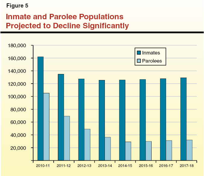
The CDCR “Blueprint.” In April 2012, the administration released a plan (commonly referred to as the blueprint) to redesign much of CDCR’s prison and parole operations in light of its significant caseload reductions under realignment. This plan included, among other changes, more standardized staffing levels across prisons, changes in how inmates are classified and assigned to different security levels of housing, elimination of the use of out–of–state contracted beds, and the closure of one prison. The plan also included the construction of three new “infill” housing units at existing prisons, as well as the renovation and conversion of a closed juvenile justice facility to a prison for adult inmates. Finally, the blueprint assumed that the administration would be able to persuade a federal three–judge panel to increase the prison population cap the panel ordered from 137.5 percent of design capacity to 145 percent. (Design capacity generally refers to the number of beds CDCR would operate if it housed only one inmate per cell and did not use temporary beds, such as housing inmates in gyms. Inmates housed in contract facilities are not counted toward the overcrowding limit.) As part of the 2012–13 budget, the Legislature approved most of the components of the blueprint requiring legislative action, including financing authority for the capital outlay projects.

LAO Forecast Assumes Implementation of the Blueprint but at 137.5 Percent Prison Cap. Our forecast generally assumes successful implementation of the CDCR blueprint. This means that there could be additional General Fund costs to CDCR if the inmate and parolee populations end up being higher than current projections or if CDCR is unsuccessful at implementing components of the blueprint expected to result in state savings. Our forecast, however, differs from the blueprint by assuming that the federal three–judge panel does not approve the administration’s plan to seek an increase in the court–ordered prison population cap to 145 percent of design capacity. (We discuss the most recent court developments on this issue in the nearby box.) Consequently, our forecast assumes that about 10,900 inmates will be housed in out–of–state contracted beds in order meet the court–ordered prison population limit. In total, we forecast CDCR General Fund expenditures to decline by about $300 million from the 2012–13 level due to projected caseload changes and implementation of the blueprint. These savings are somewhat offset by an additional $155 million annually to operate a new prison complex in Stockton designed to improve the provision of inmate health care.

Judicial Branch

We estimate that General Fund spending for the support of the judicial branch in the current year will be about $730 million, roughly $500 million lower than the amount in 2011–12. This reduction reflects budget actions to reduce General Fund support for the branch and offset most of the reduction to the trial courts with the one–time use of funds from a court construction account and trial court reserves. Beginning in the budget year, we estimate that General Fund support for the judicial branch will be about $1.2 billion, similar to the 2011–12 level. This reflects (1) the restoration of $419 million of the current–year reductions (leaving a net $71 million in ongoing unallocated cuts to the trial courts); (2) additional costs of $35 million beginning in 2013–14, growing to over $50 million annually, for service payments for the Long Beach Courthouse currently under construction; and (3) over $10 million annually beginning in 2013–14 to hold parolee revocation hearings, a responsibility that will be shifted to the courts from the Board of Parole Hearings pursuant to the 2011 realignment legislation.

Other Programs

Redevelopment Dissolution

The state’s 2012–13 budget package assumed that the General Fund would save about $3.2 billion in school funding expenses due to the dissolution of local redevelopment agencies (RDAs), as described below. Currently, we estimate that this savings will total about $1.4 billion—$1.8 billion less than assumed in the budget. Additional savings will benefit the General Fund annually in the future, such as the $1.1 billion we project for 2013–14. As discussed below, all estimates related to RDAs are subject to considerable uncertainty and are likely to change significantly between now and the deadline for adopting the 2013–14 budget in June 2013.

Background. As the operations of former RDAs wind down, their resources are being redistributed to other local agencies (cities, counties, special districts, schools, and community colleges). These resources include (1) property tax revenue not needed to pay RDA debts (residual property tax revenue) and (2) unencumbered RDA cash and other liquid assets. (Distribution of the proceeds from the sale of some former RDA real estate holdings may occur at a future date.) County auditor controllers distribute these RDA resources to local agencies in a manner similar to how they distribute property tax revenues. Most of the RDA resources provided to K–14 districts offset required state General Fund education spending, thereby creating savings for the state.

Residual Property Tax Revenue. Our forecast estimates that 2012–13 state savings from the distribution of residual property tax revenues to schools will be around $700 million. This is about $1 billion less than assumed in the 2012–13 budget. Our lower estimate is based on several factors:

• Distributions made to K–14 districts this summer were significantly lower than expected.
• Recent information suggests that RDA debts are higher than was anticipated.
• K–14 districts’ proportionate share of residual property taxes is lower than was expected.
• Some residual property taxes are distributed to K–14 districts that do not receive state funding for apportionments (so–called “basic aid districts”). These residual property taxes do not offset state education costs.

We estimate state savings from residual property tax distributions in 2013–14 will be about $500 million. These savings should grow over the forecast period, climbing to about $900 million by 2017–18. For the next several years, we anticipate that the funding needed to pay RDA debts will remain relatively flat. For this reason, growth in residual property taxes will be driven primarily by growth in former RDA property tax revenues.

Liquid Assets. Our forecast assumes that the state will realize total one–time savings of about $1.3 billion from the distribution of former RDA liquid assets to K–14 districts, including about $700 million in 2012–13 and about $600 million in 2013–14. Our projected savings for 2012–13 are about $800 million lower than assumed in the budget package.

Uncertainties Abound. We caution that our estimates are subject to significant uncertainty and could vary by several hundred million dollars annually, with a somewhat greater chance of savings being below our estimates than above them. Several factors contribute to the difficulty of developing an accurate estimate. First, although the data used to develop our estimates are the best currently available and include some reports not available at the time the 2012–13 budget was adopted, the data are very limited. Second, the willingness of RDA successor agencies—the entities overseeing the dissolution of the agencies—to comply with state direction regarding redevelopment dissolution has been uneven. Finally, the outcomes of current and expected future litigation regarding RDA dissolution could affect state savings.

Employee Compensation

The 2012–13 budget package directs the administration to achieve over $400 million in General Fund savings through the collective bargaining process, furloughs, and existing administrative authority. To achieve these savings, the administration (1) negotiated a Personal Leave Program (PLP) with most bargaining units, (2) extended the PLP to excluded employees, and (3) imposed furloughs on two bargaining units that did not agree to the PLP. Furloughs and the PLP are functionally the same policy—for the 12 months of 2012–13, employees’ pay is reduced by about 5 percent in exchange for one day off each month.

Increased Costs Beginning in 2013–14. Our forecast assumes that state General Fund employee compensation costs will increase by more than $750 million beginning in 2013–14. This amount reflects:

• The scheduled end to the PLP and furloughs in June 2013 ($401.7 million).
• An increase of between 3 percent and 5 percent in the top step of the salary range for 15 bargaining units and most excluded employees in July 2013 as specified in current law ($210 million). The state’s six other bargaining units received similar pay increases pursuant to their memoranda of understanding (MOUs) in 2012.
• Increases in the premium costs for state employees’ health care benefits averaging about 9 percent ($136 million). The California Public Employees’ Retirement System (CalPERS) negotiates health premium rates each year. We expect health premiums to continue increasing at a rate exceeding inflation for the foreseeable future.Our forecast does not include any change in state costs associated with new MOUs that could be approved by the Legislature in the future for the 20 bargaining units with MOUs that expire during the forecast period.

Future Costs of Unused Leave Uncertain. Over the years, many state employees have carried large balances of unused vacation and other types of leave. These leave balances grew significantly recently in part because of the state’s furlough and PLP policies. When an employee retires or leaves state service, the state must compensate the employee for this leave balance (“cashing out”) or allow him or her to draw pay without working (“burning off” the leave balance). Either of these two methods can result in additional state costs. The state budget process does not systematically augment departments’ budgets to cover such additional costs when they arise. Accordingly, our forecast does not assume any increased state costs associated with these leave balances. Nevertheless, in some cases, the Legislature has augmented departmental budgets for extraordinary leave balance or similar costs in order to prevent an erosion of funding available for state services. Such augmentations hypothetically could total tens of millions or hundreds of millions of dollars in any year during our forecast period, thereby increasing General Fund expenditures above the level that we are forecasting.

Retirement Benefit Costs

Pension Legislation to Result in Some State Savings. Our forecast considers the savings in state employer pension contributions that are expected to result from this year’s major pension legislation, Chapter 296, Statutes of 2012 (AB 340, Furutani). In the near term, these savings will result primarily from the legislation’s mandated increase in employee pension contributions by various groups of state employees. These increases were intended to bring these state employees’ pension contributions up to the new statewide “standard” of a 50/50 employer/employee split of pension “normal costs” (the amounts that need to be set aside each year and invested in order to cover all future costs of benefits earned in that year by employees). Our forecast relies on preliminary actuarial estimates of AB 340’s effects by CalPERS.

In part because of AB 340, our forecast assumes that General Fund state pension contributions for state and CSU employees remain relatively flat through 2017–18 at around $2.2 billion per year. Implicit in this rough estimate is an assumption that state employee salaries will remain fairly flat throughout the period (except for salary increases in already–approved labor agreements) and that CalPERS will hit its annual target for 7.5 percent investment return. Moreover, our forecast assumes no changes in CalPERS’ current actuarial assumptions, including its investment return assumptions, its existing methods for “smoothing” investment losses over many years, and its current method of “pooling” together assets and liabilities related to the pensions of past, current, and future state employees. Changes in these assumptions would tend to increase state costs noticeably if they occur during our forecast period.

Retiree Health Costs Continue to Climb Rapidly. The state pays its unfunded health and dental benefit liabilities for retired state and CSU employees as they become due—when the retirees’ benefit premiums have to be paid. This means that retiree health and dental benefits earned years—or even decades—ago by past employees are paid years later by taxpayers who may not have benefited directly from the employees’ past service. The resulting costs are much higher than if the normal costs for these benefits had been contributed and invested earlier. As more and more retirees have left state service and are living longer than prior retirees, these costs have been a rapidly growing part of the state budget for some time. They will remain so. Our forecast assumes that the combination of health premium increases and the growth of the retiree population will cause expenditures from the General Fund retiree health expenditure item to grow from $1.6 billion in 2012–13 to $2.7 billion in 2017–18—an average annual growth rate of 11.9 percent. (Around 40 percent of these General Fund costs eventually are offset by pro rata and cost recovery payments from special and other funds. These figures do not consider the “implicit subsidy” the state provides to retiree health premiums through its contributions to active employees’ benefits.)

CalSTRS Liabilities Are a Serious Long–Term Fiscal Issue. State, school district, and teacher contributions to the California State Teachers’ Retirement System (CalSTRS) for pension benefits are set in state law. In general, CalSTRS’ governing board has no power to adjust these contributions, despite the fact that the statutory stream of payments from these sources will not be sufficient to fund benefits over the long term. Our forecast assumes that the state’s current–law payments to CalSTRS remain relatively flat in the near term at about $1.4 billion per year due to the effects of recently constrained school district budgets on teacher payroll. By 2015–16, our forecast assumes that current–law payments to CalSTRS will begin to grow steadily, reaching $1.6 billion by 2017–18. Over the entire forecast period, we forecast an average annual growth rate of 3.5 percent per year.

Because our forecast assumes only current–law state payments to CalSTRS, it assumes no additional costs or policy changes to preserve CalSTRS’ solvency. Substantial additional contributions from some source will be required to address CalSTRS’ unfunded liabilities and the resulting issues for the system’s long–term solvency. Alternatively (or in addition to these higher contributions), benefits for future teachers could be reduced further (in addition to the changes in AB 340) and the resulting savings could be redirected to cover the system’s unfunded costs.

Debt Service on Infrastructure Bonds

The state uses General Fund revenues to pay debt–service costs for principal and interest payments on two types of bonds used primarily to fund infrastructure—voter–approved general obligation bonds and lease–revenue bonds approved by the Legislature. We estimate that General Fund costs for debt service on these bonds will be $5.1 billion in 2012–13, which is roughly equal to the state’s General Fund debt–service costs every year since 2009–10. General Fund debt–service costs have not increased significantly over this period for a few reasons. Most notably, the Legislature and Governor enacted legislation to permanently offset some General Fund debt–service costs with transportation funds. The 2012–13 budget package also achieved savings over three fiscal years by offsetting housing debt–service costs with proceeds from the National Mortgage Settlement. Additionally, the administration slowed the pace of bond sales over the last two years.

Over the forecast period, however, General Fund debt service is projected to grow 7.8 percent annually, reaching $7.4 billion by 2017–18. Projections of debt–service costs depend primarily on the volume of future bond sales, their interest rates, and their maturity structures. The exact timing of bond sales depends upon when various programs will need bond funds and the accessibility of financial and credit markets. In general, our forecast assumes that the slower pace of bond sales continues for many programs because they currently have sufficient bond proceeds to cover their spending needs during the initial portion of the forecast. Nonetheless, over the entire forecast period, we assume that a total of about $34 billion of already authorized general obligation and lease–revenue bonds will be sold as currently approved projects move forward. A large share of this—about $25 billion—is from the nearly $54 billion in infrastructure bonds authorized by voters in 2006 and 2008. We also expect that transportation debt–service costs will exceed available transportation funds during the forecast period and the General Fund will pay the remaining costs. Our forecast is based on the expected sale of bonds that have already been authorized, but does not include any additional bonds that may be authorized by the voters or Legislature during the forecast period.

Debt–Service Ratio (DSR) Expected to Remain Around 6 Percent. The DSR for general obligation and lease–revenue bonds—that is, the ratio of annual General Fund debt–service costs to annual General Fund revenues and transfers—is often used as one indicator of the state’s debt burden. There is no one “right” level for the DSR. The higher it is and more rapidly it rises, however, the more closely bond raters, financial analysts, and investors tend to look at the state’s debt practices and the more debt–service expenses limit the use of revenues for other programs. Figure 6 shows what California’s DSR has been in the recent past and our DSR projections for the forecast period. We estimate that the DSR will remain around 6 percent throughout the forecast period. This is because General Fund debt service and General Fund (including EPA) revenues are expected to grow at similar rates. To the extent additional bonds are authorized and sold in future years beyond those already approved, the state’s debt–service costs and DSR would be higher than projected in Figure 6.

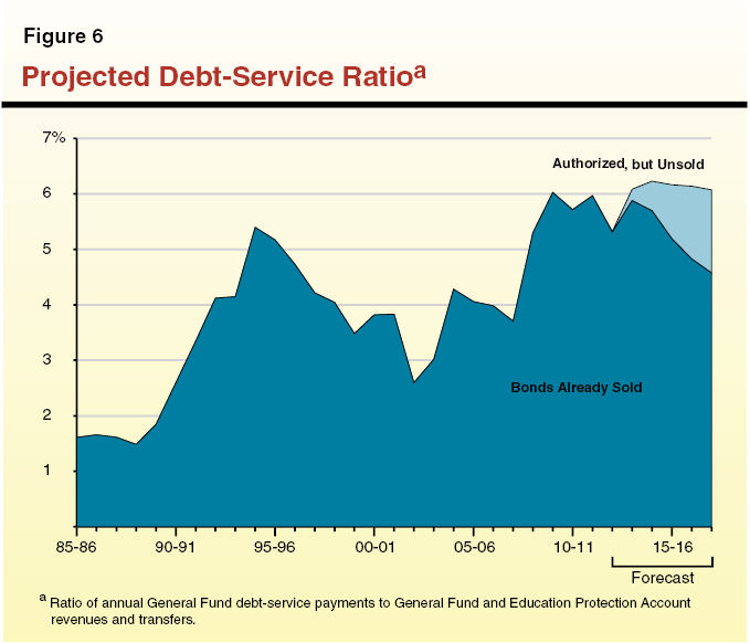
Unemployment Insurance (UI)

Interest Payments on Federal Loan. California’s UI Trust Fund has been insolvent since 2009, requiring the state to borrow from the federal government to continue payment of UI benefits. California’s outstanding federal loan is estimated to be $10.2 billion at the end of 2012. The state is required to make annual interest payments on this federal loan. These interest costs total $308 million in 2012–13. The budget authorizes this interest payment from the General Fund. To offset this cost, the budget provides a loan of a like amount from the Disability Insurance Fund to the General Fund. Based upon the Employment Development Department’s projections of the future unemployment rate, benefit payments, and UI Trust Fund revenues, we project that the General Fund annual interest payments on the outstanding loan principal will gradually decline each year from $308 million in 2012–13 to approximately $200 million in 2017–18.

Our projections for the interest payments from the General Fund do not incorporate any potential actions, such as an increase in UI taxes or decrease in benefits, that could be taken during the forecast period to address the underlying UI Trust Fund insolvency and reduce the state’s interest payment obligation to the federal government. For forecast purposes, we also do not assume that the General Fund interest obligation would be met in future years by creating new alternative funding sources or through additional special fund loans to the General Fund (although there is the potential for such actions). We note, however, that pursuant to federal law and beginning in tax year 2011, the federal unemployment tax credit for which employers are eligible (up to 5.4 percentage points of the total 6 percent tax on employee wages up to $7,000) is incrementally reduced for each year that the state continues to have an outstanding federal loan to the UI Trust Fund. The increase in federal unemployment taxes paid by California employers due to the tax credit reduction—approximately $290 million in 2012—is used to reduce the federal loan balance.