Ann Hollingshead

April 10, 2025
Rethinking California’s Reserve Policy
- Introduction
- Chapter 1: How Much Should the State Save in Reserves?
- Chapter 2: Where Are We Now?
- Proposition 2 Has Substantially Improved State’s Reserve Policy
- Yet Further Improvements Are Warranted
- Chapter 3: Where Do We Go from Here?
- Governor’s Proposal
- LAO Recommendations
- Conclusion
Executive Summary
Rethinking California’s Reserve Policy. Reserves allow the state to ensure stable funding for its services over time, even when revenue fluctuates unpredictably. Over the last few years, the state has indeed experienced those significant fluctuations—large surpluses followed by significant deficits. This volatility has prompted interest in changes to the state’s reserve policy. The Governor has proposed two changes that, if passed by the Legislature, would go before voters. In this report, we assess those proposed changes. We find that while they would improve upon the state’s reserve policy, they would not reliably ensure stable funding for core services over time, and therefore further changes are warranted. As such, we examine how much the state would need to save in reserves to maintain its core services during future downturns.
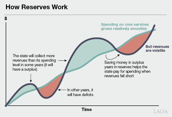
What Is the Purpose of Reserves? The state will collect more in revenues than the cost of its core service level in some years. In other years, it will collect less. Reserves help smooth the difference—funds are saved when revenues are surging (the green regions in the figure below) and then spent when revenues decline below that long‑term trajectory (the red regions). If reserves are insufficient to cover these shortfalls, the state must eventually: (1) raise taxes or (2) cut those services. This means that the more reserves the state has, the more it can mitigate the need for those cuts and tax increases.
How Do We Evaluate the Performance of Reserve Policies? A reserve policy “performs well” if it meets the central goal of reserves—that is, it allows the state to save enough so that the state can pay for spending on its core services when revenues drop. When revenues are insufficient for the state to pay for its core service level, we describe the difference as a funding shortfall. To evaluate how much funding shortfalls can be covered with reserves we have constructed simulation‑based tools—similar those used in insurance markets and the state’s pension system—that use information about the past to forecast many different variations of the future. We report findings across 50 years and thousands of these simulations.
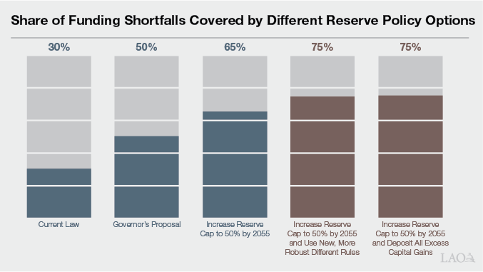
Under Current Law, the State Can Cover One‑Third of Funding Shortfalls. We find that the state’s current constitutional rules for building reserves would allow the state to cover about one‑third of funding shortfalls. Put another way, if current law remained in place for the next 50 years, and without further saving above this level, cuts to core services and/or tax increases would often be necessary.
Governor’s Proposal Improves Upon Current Law, but Further Improvements Are Warranted. The Governor proposes two changes to the state’s reserve policy: (1) raise the cap on constitutional deposits from 10 percent of General Fund taxes to 20 percent, and (2) make reserve deposits excludable from the state appropriations limit. The Governor’s proposal improves upon current law—rather than one‑third, these changes would allow the state to cover about half of funding shortfalls over 50 years. However, even with this change, reductions to core services or tax increases would still be common. In our view, this means further improvements are warranted.
LAO Recommended Approach. We put forward two recommendations to improve reserve policy:
- Raise the Reserve Cap to 50 Percent by 2055. We first recommend the cap on constitutional reserve deposits be raised from 10 percent to 50 percent of General Fund taxes. The increase could be phased in over time: 20 percent to take effect immediately after the next statewide election, 25 percent in 2030, and increasing by 5 percent every five years until the cap reaches a maximum of 50 percent in 2055.
- Two Options to Reach This Higher Threshold. If the cap is raised, the state would also need to set aside more in reserve deposits to dependably reach this higher amount. There are many options for doing this, but given the volatility in the state’s revenues, we think it is important to set aside much more funds in years when revenues are surging, rather than setting aside somewhat more in every year. We suggest two alternative mechanisms to accomplish this: (1) create new, more robust and flexible deposit rules, or (2) keep existing rules in place, but change them to set aside more in capital gains revenues in some years.
The figure below shows how the state’s reserve policy would perform under our recommended alternatives. As it shows, we estimate our recommendations would allow the state to cover about three‑quarters of funding shortfalls over the next 50 years.
These Recommendations Are an Honest Reflection of Revenue Volatility. We understand that building a reserve of this size—even if achieved over three decades—is a dramatic increase and well outside the range of savings targets that have been contemplated by policymakers to date. Yet we do not view these recommendations as overly cautious—to arrive at these estimates, we have used standard tools from actuaries in pensions and insurance markets. These problems are also clear when California’s reserves are compared to other states—California ranks near the top in terms of revenue volatility, but below average in terms of reserves. As such, our recommendations are an honest reflection of the volatility in the state’s tax system. That is, these changes would allow the state to enjoy the advantages of its current revenue structure while protecting critical services for Californians for decades to come.
Introduction
Reserves allow the state to ensure stable funding for its services over time, even when revenue fluctuates unpredictably. By setting aside funds when revenues are surging, the state can maintain core services when those revenues fall short. Reserves have become particularly salient to the budget process in recent years. After allocating surpluses totaling over $100 billion across 2021‑22 and 2022‑23, the Legislature has addressed cumulative budget problems of $82 billion in the years since. Budget problems are also likely to persist for the foreseeable future. In fact, given the scale of both actual and projected deficits, the Legislature likely faces the difficult choice about how to reduce core services in the coming years.
In light of these developments, the Legislature has signaled an interest in making changes to the state’s reserve policy. In addition, through this year’s budget process, the Governor has proposed two changes to the state’s rainy day fund that, if passed by the Legislature, would go before voters. This raises an important question: Are these changes sufficient? That is, how much does the state need to save in reserves to maintain its core services during future downturns and would the Governor’s proposal achieve that goal? If not, what is a reserve policy that would? This report aims to answer these questions by taking a long‑term view. That is, we aim to construct a reserve policy that has the best chance of withstanding the test of time and minimizes the need for the Legislature to ask voters to make further changes to the Constitution in a few years.
The report is organized as follows. Chapter 1 lays out a framework for establishing a goal for the state’s reserve policy, and then tools that can be used to estimate how much in reserves the state needs to save to achieve that goal over time. In Chapter 2, using the tools outlined in Chapter 1, we evaluate the state’s current reserve policy. Chapter 3 examines possible changes to the state’s policy, including the Governor’s proposals and our recommended alternatives.
Chapter 1: How Much Should the State Save in Reserves?
This section presents our framework for thinking about how much in reserves the state should save. First, we describe the goal of reserves. Then, we describe the ways we can quantitatively evaluate whether or not a reserve policy is meeting that goal.
What Is the Purpose of Reserves?
Revenues Are Volatile… From year to year, state revenues can grow very quickly or contract quickly. Revenues drop during economic recessions, when business activity slows, unemployment rises, and consumer spending declines, leading to lower tax collections. Asset market downturns, like stock market drops or real estate slumps, can also reduce capital gains tax revenue and other investment‑related income, lowering state revenue. Conversely, revenues can grow quickly in response to economic expansions or run ups in the stock market.
…And Core Spending Is Not. Meanwhile, the ongoing costs of state programs—the state’s core service level—is much steadier. Spending on core services can fluctuate in response to recessions, for example, because of caseload growth in means‑tested programs that occurs in response to unemployment changes. However, in general, growth in core services tracks more stable factors, like inflation (especially inflation for pharmaceuticals and health care) and population (especially in some key demographic areas). Conversely, growth in total spending—rather than spending on core services alone—does fluctuate much more. This is largely because the Legislature allocates considerable shares of revenue surges to one‑time and temporary spending.
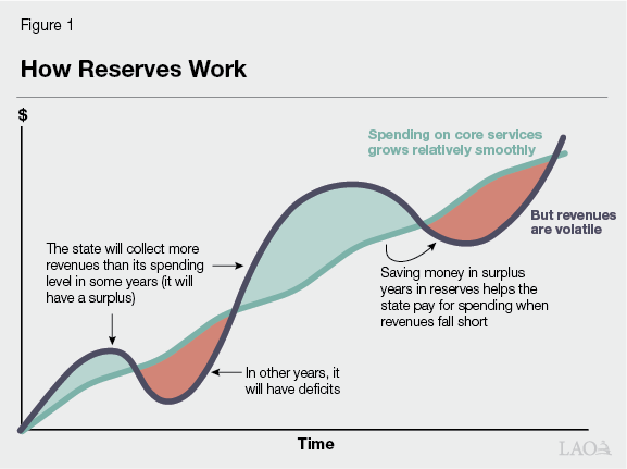
Reserves Allow the State to Smooth the Difference. The state will collect more in revenues than the cost of its core service level in some years. In other years, it will collect less. Reserves help smooth the difference. As shown in Figure 1, reserves can be saved when revenues are surging (the green regions) and then spent when revenues decline below that long‑term trajectory (the red regions). Importantly, this hypothetical—and the estimates of core services in this report—only speak to reserve policy on one side of the budget, that is, excluding the budget devoted to schools and community colleges. The nearby box describes why this is our focus.
Reserve Policy and the Two Sides of the State Budget
State Budget Can Be Thought of in Two Distinct Parts. Functionally, California’s General Fund budget is divided into two parts: one dedicated to K‑14 education (about 40 percent of the total) and another part that funds everything else (roughly 60 percent of the total). The reason for this bifurcation is Proposition 98 (1988), which requires the state to set aside minimum amounts of funding for schools and community colleges. With rare exceptions, the state must fund this baseline regardless of other budget pressures. As a result, Proposition 98 creates a separate budget for K‑14 education that sits within the state’s larger budget.
Budget Conditions Can Diverge. The budget situation within Proposition 98 can diverge sharply from the rest of the budget. For example, there can be a “surplus” within the Proposition 98 budget (meaning that funding under the guarantee is more than sufficient to cover the costs of existing educational programs) even as the rest of the General Fund faces a deficit. That said, the conditions of these two parts of the budget tend to move together because, under the constitutional formulas, funding for schools and community colleges will usually decline in response to drops in revenues.
Schools and Community Colleges Have Separate System to Mitigate Revenue Volatility. Revenue volatility is an issue for both sides of the budget, but each side also has distinct and dedicated policies to address that volatility. For schools and community colleges, the main tool is the state’s Public School System Stabilization Account (the Proposition 98 Reserve), which requires the state to save more in reserves when revenues—especially those from capital gains taxes—are surging. These funds must be used to supplement, but not supplant, Proposition 98 spending during a downturn. In addition, school and community college districts themselves hold local reserves to manage unexpected cost increases, as well as state funding declines. Finally, the state has used other tools like deferrals, which uses a principle similar to borrowing to help smooth school spending through downturns.
This Report Does Not Address Reserve Policy for Schools. Given the division of the budget and the separate reserve policies in place for schools and community colleges, this report focuses only on the reserve policy for the rest of the budget. That is, the recommendations and estimates in this report only address revenue volatility for the side of the budget that does not include schools and community colleges, and this report does not speak to the adequacy of preparedness for the Proposition 98 budget for revenue downturns.
Reserves Allow the State to Avoid Tax Increases and Cuts to Core Services. The State Constitution requires the Legislature to pass a balanced budget. So, if the state does not have enough reserves to cover shortfalls between revenues and spending on core services, the state must eventually: (1) raise taxes or (2) cut those services. (The state also has the option borrow or shift costs to address deficits, but only on a limited and temporary basis. Functionally, borrowing has the same impact as reserves—it moves money from a period when state revenues are surging to one when they fall short—but generally involves higher interest costs for the state. The main difference, however, between reserves and borrowing is that the former involves setting aside funds up‑front whereas the latter would fund a deficit after the fact.) The more reserves the state has, the more it can mitigate the need for spending cuts or tax increases.
Revenue Downturns Will Occur, the Question Is When. The state’s revenue fluctuations are often described in terms of risk, like a car owner protecting against the risk of an accident or a corporation hedging against the risk of changes in sales. A more risk‑averse car owner might purchase full‑coverage insurance while a less risk‑averse car owner might purchase only what is legally required. Yet these analogies do not well describe the state’s revenue situation—because, unlike with a car accident, the question of revenue drops is not if but when. That is: the state will face revenue downturns in the future, but we can’t predict when those will occur or how big they will be. This makes the state’s reserve policy more like an individual saving for retirement. A person saving for retirement does not know how long they will live or exactly what their expenses will be in retirement, but they nonetheless must plan for this eventuality by making the best possible choices in the meantime. That person might experience annual fluctuations in their financial situation that causes them to save more or less in any given year. However, their long‑term plan should be constructed irrespective of these annual fluctuations. This analogy can be easily extended to the state’s reserve policy, which can fluctuate from year to year but should be constructed by examining a very long‑time horizon in order to facilitate the stable provision of services.
How Do We Evaluate Reserve Policies?
We Use Simulation‑Based Tools Similar to Those Used to Analyze Pensions and Insurance. The state’s reserve policy should hold up not just for a few years or even a couple of decades, but over many economic cycles. In this report, we test reserve policies over 50 years. On an analytical basis, there is nothing inherently correct about this time frame, except that it is long enough to allow us to measure the cumulative effect of several economic cycles. Predicting the exact path revenues will take over the next 50 years is, of course, impossible. However, we can make informed estimates about the future with tools similar those used in insurance markets and the state’s pension system. Similar to actuaries in these fields, we have constructed simulation‑based tools that use information about the past to forecast many different variations of the future. With these scenarios in hand, we can then measure how well a reserve policy performs in not just one or two scenarios, but thousands of them.
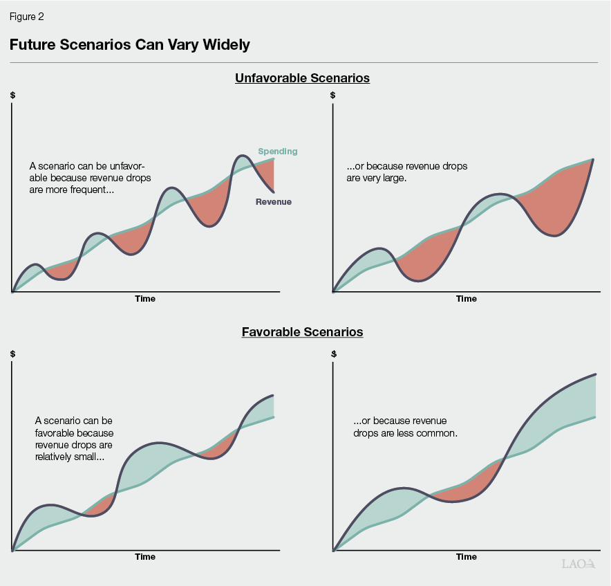
What Are These Scenarios? Each of these scenarios draws on data from the past—like long‑term growth rates and the stability and the persistence of past trends—to make predictions about the future. However, each individual scenario is also unique. That is, it will look different than the past and all the other scenarios. Some scenarios are unfavorable ones, while others are more favorable (see Figure 2). In an unfavorable scenario, for example, the state could face a series of more moderately sized recessions in close proximity to one another. Or, in a very unfavorable scenario, the state could encounter three Great Recessions over the course of five decades. Conversely, in more favorable scenarios, the state might only face a series of mild to moderate recessions, spread far apart over the 50 years.
Choosing the Right Benchmark Scenario. We do not know which of these scenarios will be the state’s actual future (or if the future will hold something else, entirely outside of the scope of our scenarios). If the Legislature adopts a reserve policy that performs well in half of scenarios but poorly in the other half (that is, we use the median scenario as a benchmark), it would mean there is something like a coin‑flip chance that the policy would achieve its desired outcomes. It is reasonable therefore to choose a policy that performs well across the substantial majority of scenarios. For our analysis, we use the 90th percentile as our benchmark—that is, we measure the effectiveness of various reserves policies according to how well they do in some of the most unfavorable scenarios, but not the absolute worst. At this level, we can be reasonably confident a particular policy will have its intended impact. Using outcomes from unfavorable scenarios to make policy recommendations is a standard practice for actuaries in fields like pensions and insurance.
How Do We Measure the Core Service Level? In addition to simulating revenues, this analysis requires us to define the state’s core service level. This is an inherently subjective concept, in part because “core services” are not immutable. Instead, core services will change over time as the state responds to changes in revenues by expanding or contracting the size of government. While a portion of temporary surges in revenue will be allocated to one‑time spending, after a period of time, the Legislature will begin to expand service levels in response to sustained revenue growth. As such, we approximate “core service level” using the three‑year moving average of enacted revenues, frozen in the year before a revenue decline begins. While this may be somewhat counterintuitive, this method captures the fact that core services are a dynamic concept. This method also accounts for the fact that, due mainly to other constitutional spending requirements, revenue losses do not result in deficits on a 1:1 basis. This is in particular due to Proposition 98 (1988), in which required spending on schools and community colleges tends to fall when revenues decline.
A Reserve Policy Performs Well if It Allows the State to Pay for Core Services During a Revenue Drop. Using these estimates of core spending and revenues in the benchmark scenario, we then evaluate how well various reserve policies perform. Specifically, a reserve policy “performs well” if it meets the central goal of reserves—that is, it allows the state to save enough so that the state can pay for spending on its core services when revenues drop. In this report, when revenues are insufficient for the state to pay for its core service level, we describe the difference as a funding shortfall. A funding shortfall is distinct from a budget deficit, which occurs when revenues are insufficient for the state to pay for all of its currently authorized services (not just core services). The nearby box describes this difference in more detail.
Funding Shortfall Versus Budget Deficit
A budget deficit occurs when revenues are insufficient to pay for all of the state’s enacted programs—including both core services and newly enacted or temporary programs. Because of the state’s balanced budget requirement, a deficit must be closed before a budget can be enacted. A deficit is related to, but distinct from, the concept of a funding shortfall described in this report. The key conceptual difference is that a budget deficit will include the effects of recently enacted one‑time and temporary spending augmentations, whereas our aim in measuring the state’s funding shortfall is to isolate the costs of the state’s core service level. Further, budget deficits are highly influenced by estimation error and our method abstracts away from these year‑by‑year particularities. Overall, we would describe funding shortfalls, as measured in this report, as considerably smaller than budget deficits.
Analyzing the State’s Reserve Policy. Throughout the remainder of this report we analyze different policy alternatives based on how well they perform on the criteria we have outlined here. That is: over a fifty‑year period, we measure the share of funding shortfalls that the state can cover with reserves under different policies, considering scenarios that are unfavorable, but not the worst possible. In other words, this is our assessment of the reserves that are needed for the state to maintain its core service level over time without cutting core services or raising taxes.
Chapter 2: Where Are We Now?
In 2014, voters approved significant reforms to the state’s reserve policy with Proposition 2. This measure substantially improved the state’s reserve policy, particularly relative to recent history. However, using the tools described in Chapter 1, this policy falls well short of the amount of reserves that are needed.
Proposition 2 Has Substantially Improved State’s Reserve Policy
Before 1980, State Reserves and Surpluses Varied Widely. Before the 1980s, the state’s budget was enacted with either a year‑end surplus or deficit (at this time, the state had no balanced budget requirement). These balances would roll forward into the next year’s budget, and therefore surpluses would provide a buffer against revenue declines, but they were not explicitly earmarked for this purpose. To deal with unexpected budget shortfalls, the state also created a reserve fund—the Revenue Deficiency Fund—in 1947. The fund initially received a balance of $75 million, representing about 14 percent of the budget at the time. The $75 million balance remained until it was withdrawn roughly a decade later. In this period, state surpluses also varied widely, as shown on the left side of Figure 3. In the 1950s, the state had significant reserves and surpluses (the amounts in Figure 3 are additive, so in the 1949‑50 budget, reserves and surpluses represented 42 percent of revenues). In the late 1970s, the state had sizeable surpluses, but no reserves on hand.
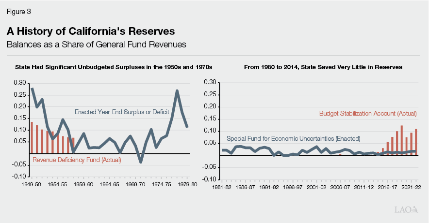
Proposition 4 (1979) Required California Governments to Establish Reserve Accounts. Partially motivated by the budget surpluses of the late 1970s (but not reserves, as the state had none), voters passed Proposition 4 in November of 1979. This measure placed limits on how much tax revenues governments in California could spend. (At the state level, this is referred to as the state appropriations limit [SAL]. The measure is also referred to as the “Gann limit,” named after one of its authors.) In addition to establishing these spending limits, Proposition 4 suggested each entity of government establish a contingency or reserve fund in the amount “deemed reasonable and proper” and requires deposits into these funds to be treated as spending subject to the limit. In response, the state created the contingency reserve for economic uncertainties—a precursor to what is now the Special Fund for Economic Uncertainties (SFEU). The balance of the SFEU is determined by the annual budget act and essentially functions like the ending fund balance of the General Fund. The SFEU is therefore somewhat akin to the year‑end unallocated surpluses of the 1950s through 1970s.
Before 2014, State Had Very Little in Reserves on Hand. After the 1980s, but prior to 2014, the SFEU was nearly exclusively used as the state’s budget reserve. Throughout this period, as shown on the right side of Figure 3, the SFEU balance was generally enacted around 1 percent to 3 percent of revenues—very small compared to the reserves and surpluses of the decades before. There was only one brief departure from this paradigm. In March of 2004, on the heels of the dot‑com bust, voters passed Proposition 58, which created the Budget Stabilization Account (BSA). In the 2006‑07 budget, the Legislature deposited $472 million into the BSA and in 2007‑08 deposited $1.5 billion. However, in the early months of the Great Recession, the state acted quickly to withdraw all of these funds. This meant California weathered most of the Great Recession with essentially no reserves on hand.
Proposition 2 Substantially Improved State’s Reserve Policy Relative to Recent History. In response to the state’s significant budget problems during the Great Recession, voters passed Proposition 2 in 2014, making significant changes to the state’s reserve policy. These changes included: (1) new rules for deposits into the BSA, (2) limitations on the Legislature’s ability to access the fund, and (3) a new maximum level for constitutional deposits into the fund. (Proposition 2 also created the Proposition 98 Reserve, which was discussed in the box previously.) After Proposition 2 was passed, the state saved significantly more in reserves, particularly when compared to the savings levels from the early 1980s through the early 2010s. That said, in percentage terms, the BSA balance is comparable to—perhaps even a bit smaller than—the Revenue Deficiency Fund of the 1950s. (At its largest, the BSA reached 12 percent of General Fund revenues, while the Revenue Deficiency Fund was initially set at 14 percent of General Fund revenues.)
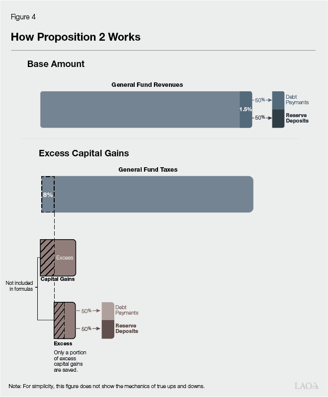
How Does Proposition 2 Help the State Build Reserves? Figure 4 shows how Proposition 2 deposit rules work. The measure has two main parts. First, it requires the state to set aside 1.5 percent of total General Fund revenues (we refer to this as the “base amount”). Second, it requires the state to set aside a portion of capital gains revenues that exceed 8 percent of General Fund taxes (this is: “excess capital gains”). Importantly, the state does not set aside all capital gains that exceed this threshold, but only a share of them. This share is determined by a complex set of formulas that can lower excess capital gains by anywhere from 0 percent to 100 percent, although reductions around 30 percent have been the most common to date. The state combines the base and excess capital gains amounts and allocates half to pay down debts and the other half to build the rainy day reserve.
State Has Neared or Reached the BSA Cap Twice. Proposition 2 limits how much can be saved in the constitutional reserve to 10 percent of General Fund taxes. (There is no limit on how much can be saved on a discretionary basis.) Currently, this is about $21 billion. Once the BSA reaches this level, any deposits otherwise required must instead be spent on infrastructure. While the state neared this cap in the 2019‑20 budget, the cap has only been operative twice: in 2022‑23 and 2023‑24. All told, had there not been a cap on constitutional deposits, the state would have deposited about $2 billion more in reserves.
Suspensions and Withdrawals Have Occurred Infrequently. In addition to creating new rules for reserve deposits, Proposition 2 created new rules regarding when otherwise‑required deposits can be suspended and when funds can be withdrawn from the BSA. Specifically, suspensions or withdrawals can only occur if the Governor declares a budget emergency. The Governor may call a budget emergency in two cases: (1) if estimated resources available in the current or upcoming fiscal year are insufficient to keep spending at the level of the highest of the prior three budgets, adjusted for inflation and population (a “fiscal emergency”), or (2) in response to a natural or man‑made disaster. (Under the language of Proposition 2, “resources available” includes both revenues and the entering fund balance.) Since 2014, the state has suspended and made withdrawals from the BSA in two years: 2020‑21 and 2024‑25. In addition, there is a withdrawal planned for 2025‑26 under legislative action taken last year.
State Has Made Some Discretionary Reserve Deposits. In addition to what has been required under Proposition 2, since 2014, the Legislature has at times made discretionary reserve deposits. For example, in 2018‑19, the Legislature created the Budget Deficit Savings Account—which was used to temporarily hold a $2.6 billion optional deposit into the BSA—and the Safety Net Reserve—a reserve specifically dedicated to CalWORKs and Medi‑Cal. The Safety Net Reserve initially received a deposit of $200 million and the balance of the fund eventually grew to a $900 million.
Yet Further Improvements Are Warranted
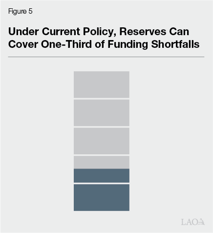
Proposition 2 Only Allows the State to Cover About One‑Third of Funding Shortfalls. We have evaluated the effectiveness of Proposition 2 using the simulation‑based tools described in Chapter 1. We find that, under current law, the reserves built under Proposition 2 allow the state to cover about one‑third of funding shortfalls (see Figure 5). Put another way, if Proposition 2 remained in place as is for the next 50 years, in the benchmark scenario, the state would be able to cover about one‑third of funding shortfalls such that cuts to core services and/or tax increases would often be necessary. This has been relatively apparent from recent history, as well. Although the state had surpluses that totaled over $100 billion across 2021‑22 and 2022‑23, Proposition 2 required only a about $10 billion to be saved over a similar period. Further, since 2023‑24, the Legislature has addressed $82 billion in budget problems (with more in deficits likely to emerge in the coming years), but at its largest, the BSA balance reached only $23 billion.
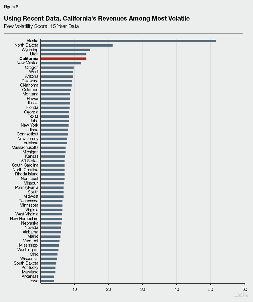
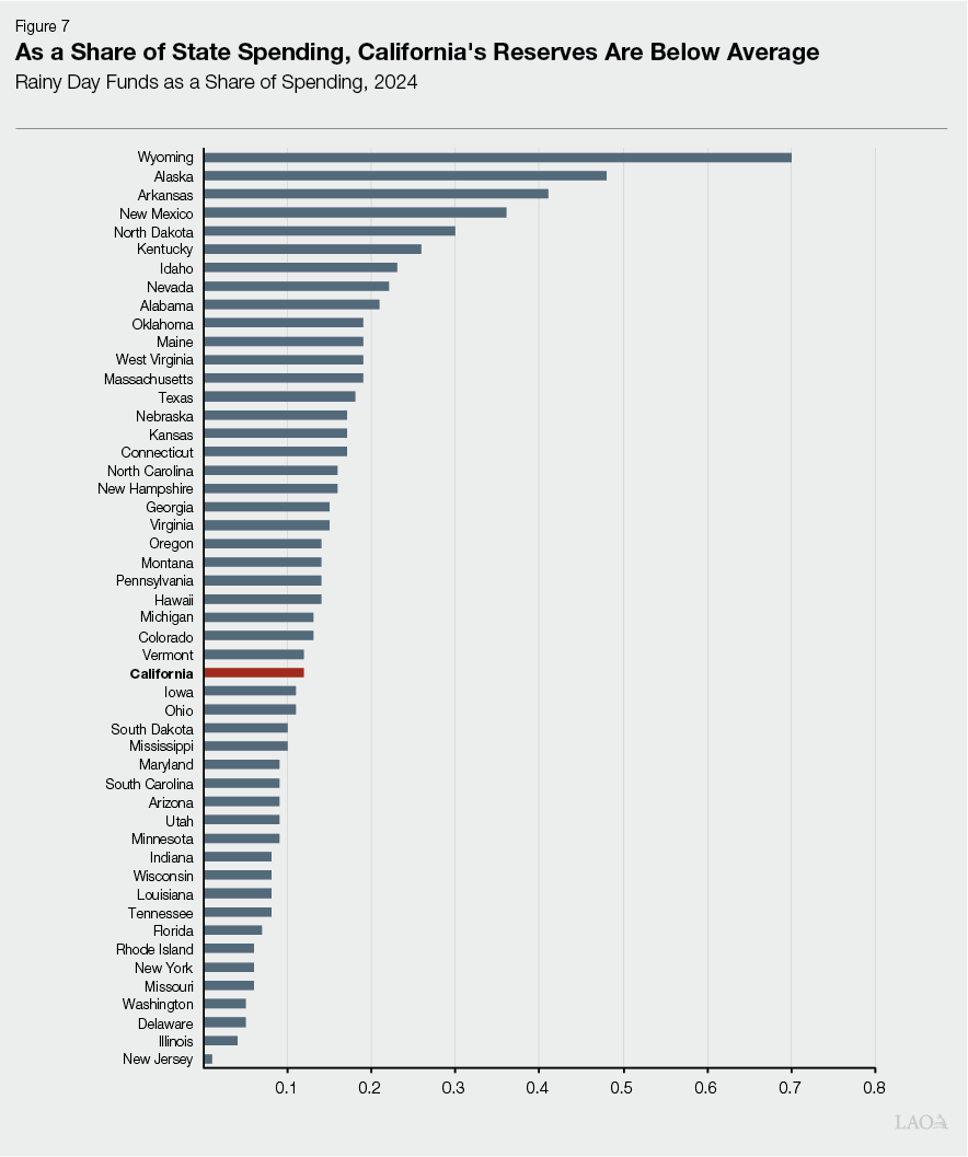
Compared to Other States, Revenue Volatility Is High, but Reserve Balances Are Relatively Low. Comparing California’s current reserve policy to other states offers another perspective on the shortcomings of Proposition 2. Figure 6 shows a measure of state revenue volatility put together by researchers at the Pew Charitable Trusts using 15 years of revenue collection data. According to this measure, California has one of the most volatile tax revenue systems in the country, ranking fifth out of 50 states. However, using data from the Fiscal Survey of States put together by the National Association of State Budget Officers, California’s rainy day fund balances are somewhat below average. Figure 7 shows states’ rainy day funds as a share of total spending in 2024. On this measure, California’s reserves rank 29 out of 50. (In fact, Figure 7 likely overstates California’s reserve balances compared to other states because the data appears to include the SFEU in the state’s rainy day fund balances, although it is not a true rainy day fund.)
Chapter 3: Where Do We Go from Here?
In this section, we evaluate the Governor’s proposed changes to Proposition 2 using the tools described in Chapter 1. We find that while they would improve upon the state’s reserve policy, they would not reliably ensure stable funding for core services over time, and therefore further changes are warranted. As such, this section also presents our proposed alternative—new rules for reserve deposits that would allow the state to save enough in reserves to maintain its core services during future downturns.
Governor’s Proposal
Governor Proposes Two Changes to Proposition 2. The Governor’s budget includes proposed trailer bill language that would put a measure before voters to make two changes to Proposition 2. Those are:
- Raise BSA Cap to 20 Percent of General Fund Taxes. The Governor proposes raising the reserve cap from 10 percent of General Fund taxes to 20 percent of General Fund taxes. This would not have any impact on the rules that set aside funds each year, but would mean the state would save more cumulatively over time.
- Exclude BSA Deposits From the SAL. The Governor also proposes excluding BSA deposits from the SAL. (Reserve withdraws are already excluded and the Governor does not propose changing that.) This proposal does not impact the constitutional deposit rules, but it could make it easier for the state to save more on a discretionary basis in certain years. (It would also somewhat reduce the budgetary constraints created by the SAL in certain years.)
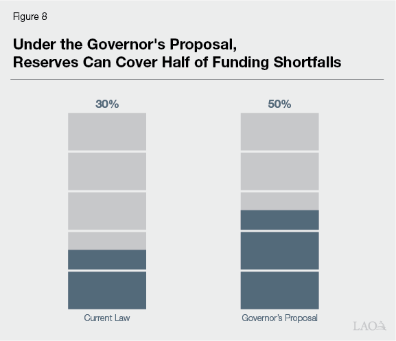
Raising the Reserve Cap Improves Upon Current Law, but Further Improvements Are Warranted. Figure 8 uses the tools described in Chapter 1 to evaluate the Governor’s proposal. The Governor’s proposal clearly improves upon current law. In particular, in the benchmark scenario, the Governor’s proposal would allow the state to cover about half of funding shortfalls over 50 years. (This analysis assumes that, after 2029‑30 when debt payments become optional, the state dedicates all of the Proposition 2 requirements to reserves, rather than splitting those requirements between reserves and debt.) Although this is a clear improvement over current law, it also implies that, even under the Governor’s proposal, either reductions to core services or tax increases would still be common. In our view, this means more improvements are warranted.
Excluding Reserve Deposits From SAL Has Merit. While Proposition 2 requires the state to set aside minimum amounts in reserve each year, Proposition 4 treats reserve deposits like state appropriations. As we have noted in the past, this creates an implicit tension between these two constitutional calculations. We think it is reasonable to ask the voters for a change to Proposition 4 to bring these measures into congruence.
LAO Recommendations
In this section, we present our recommendations for changes to reserve policy that would allow the state to cover a more substantial share of funding shortfalls in the benchmark scenario. To this end, we have two main recommendations: (1) raise the reserve cap to 50 percent by 2055 and (2) change the rules to set aside more revenues so that the state can dependably reach this higher threshold.
Raise the Cap to 50 Percent by 2055
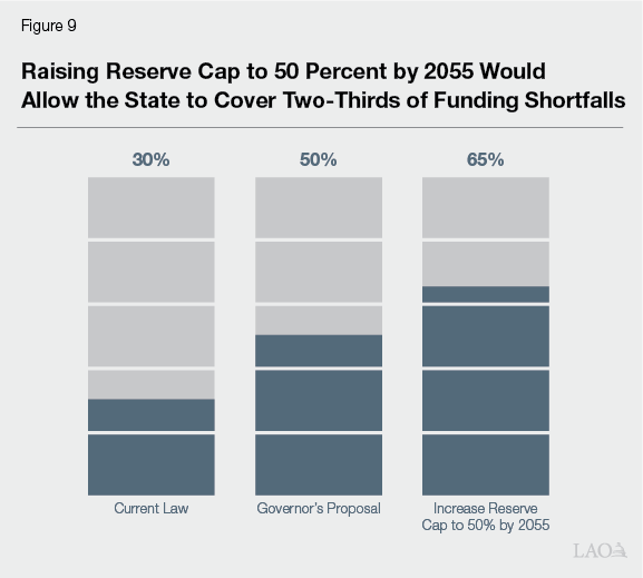
We first recommend that the Legislature raise the BSA cap to 50 percent of General Fund taxes. This change need not occur immediately as it will take time for the state to build up reserves through future economic cycles. As such, we suggest the Legislature ask the voters to authorize a scheduled, phased‑in increase: 20 percent to take effect immediately after the next statewide election, 25 percent in 2030, and increasing by 5 percent every five years until the cap reaches a maximum of 50 percent in 2055. This change alone would improve upon the Governor’s proposal considerably—under our benchmark scenario, the state would be able to cover two‑thirds of funding shortfalls across 50 years, rather than only half (see Figure 9). (Similar to the above, this analysis assumes that, after 2029‑30 when debt payments become optional, the state dedicates all of the Proposition 2 requirements to reserves, rather than splitting those requirements between reserves and debt.)
Importantly, we have found that raising the cap further than the level proposed by the Governor is the only way to substantively improve upon the proposal. That is, if the state were to raise the reserve cap to 20 percent and also increase annual deposits—for example, by increasing the base amount—it would not result in a substantial improvement in the benchmark scenario. Put another way: until it is raised substantially, the cap is the most important binding constraint on the state’s ability to build reserves.
Options to Reach This Higher Threshold
If the cap is raised substantially—ideally to 50 percent by 2055—the state would also need to set aside more in reserve deposits to dependably reach this higher amount. There are many options for doing this, but given the volatility in the state’s revenues, we think it is important to set aside much more funds in years when revenues are surging, rather than setting aside somewhat more in every year. This strategy avoids forcing the state to save more in years when the budget position is positive, but more marginal. In these years, saving more money might come at the expense of high‑priority legislative goals. Saving aggressively in strong revenue years, by contrast, helps avoid those more difficult choices. In this section, we present two alternative mechanisms for reaching a higher savings goal using this strategy.
Create New, More Robust and Flexible Deposit Rules
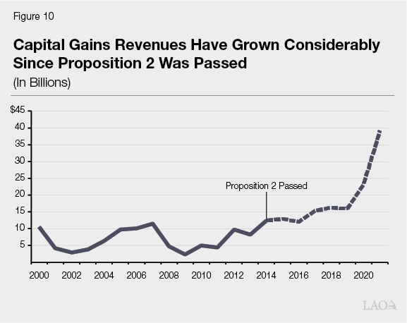
The Legislature could first consider asking voters to replace Proposition 2’s existing framework for deposit rules with something entirely different. There are several reasons this is appealing. First, the existing system is complicated and difficult for even for well‑informed budget observers to understand. Second, the existing formulas focus on capital gains as the key source of revenue volatility for the state, but increasingly, the state’s revenues have other sources of volatility, like corporation tax and even withholding in the personal income tax. Diversifying the way volatility is measured would ensure the state is capturing surges in these other revenues. Finally, capital gains revenues have grown substantially since the passage of Proposition 2 (see Figure 10) and while it is possible that this growth will persist, it is not a guarantee. Changing the structure of the rules to diversify the types of volatility considered could help insulate the reserve policy against the risk of a paradigm shift where growth in capital gains revenues is not as robust in the future.
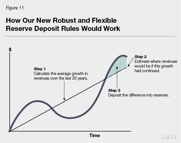
Recommended Alternative System Would Set Aside Windfalls Relative to Expectations. We suggest an alternative set of rules for deposits that uses three steps to identify and set aside windfall revenues. First, the state would calculate the average growth rate in revenues over 20 years. Second, using this growth rate, the state would estimate where revenues would be in the current year if they had grown at that rate over the past three years. Finally, the state would then deposit the difference between actual current‑year revenues and this projected amount into reserves. Figure 11 shows how these steps are calculated. The intuition of this approach is that we establish a baseline for “expected” revenue growth based on long‑term trends. Any revenues above this baseline would be considered potential windfall funds—one‑time resources that are better suited for reserves than for budget commitments.
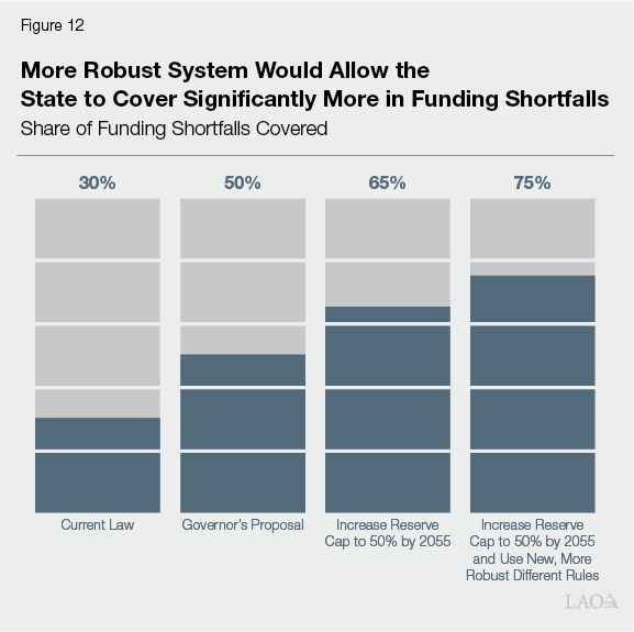
This More Robust and Flexible System Would Allow the State to Cover Significantly More in Funding Shortfalls. As Figure 12 shows, using these new, more robust and flexible rules—coupled with an increase in the reserve cap to 50 percent by 2055—the state could cover about three‑quarters of funding shortfalls over the next 50 years. An even higher share of funding shortfalls could be covered in the unfavorable benchmark scenario with even more expansive rules. However, in the course of our analysis, we found that doing so would require the state to save impractically high levels of reserves in more favorable scenarios. As such, we think a reserve policy that covers three‑quarters of funding shortfalls is adequate while balancing these trade‑offs.
Keep Existing Formulas, but Set Aside All Excess Capital Gains
Although there would be many advantages to replacing the existing Proposition 2 formulas with something simpler and more robust, we understand that it might be easier to reach agreement on reserve changes that build off existing policies rather than replace them. To this end, below we put forward an alternative to building more reserves that keeps the existing Proposition 2 deposit rule structure largely intact, but also focuses on saving more during surges in state revenues.
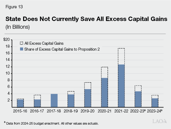
Proposition 2 Does Not Currently Save All Excess Capital Gains. Under current law, the state does not set aside all capital gains but rather a share of them based on a complicated set of formulas. Due to complex interactions, those formulas inconsistently reduce the excess capital gains directed to Proposition 2. As shown in Figure 13, since Proposition 2 was passed, excess capital gains to Proposition 2 have been reduced between 0 percent to 30 percent each year (larger increments are also possible, if not likely, in the future). For example, between 2020‑21 and 2021‑22, the formulas reduced the share of excess capital gains that benefit Proposition 2 by $8 billion.
Saving All Excess Capital Gains Would Allow the State to Save More Revenue Peaks. If the state instead saved all excess capital gains, it would mean setting aside more “peaks” in capital gains revenues. This is more appealing than making other changes to Proposition 2 rules—such as raising the base amount above 1.5 percent or lowering the threshold for excess capital gains below 8 percent. These types of other changes would not set aside more windfall revenues, but rather increase the amount that is saved every year (or most years). Setting aside all capital gains revenues would increase the state’s spending on both debt payments and reserve deposits before 2029‑30. After 2029‑30, the Legislature could choose to dedicate all of these requirements to reserves.
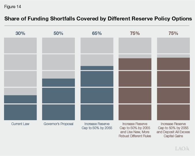
Along With Changes to Reserve Cap, State Could Cover About Three‑Quarters of Funding Shortfalls. As Figure 14 shows, by setting aside all excess capital gains—coupled with an increase in the reserve cap to 50 percent by 2055—the state could cover about three‑quarters of funding shortfalls over the next 50 years. This is essentially the same as the estimated outcome under the alternative to replace the rules with something simpler and more robust. That said, these estimates could be wrong if the future differs significantly from that past. This risk is larger for the capital gains approach—which relies on specific assumptions about inherently unpredictable capital gains—than our simpler alternative—which relies only on more general assumptions about revenue volatility broadly. As such, we view our alternative as a safer and more robust option.
Other Complementary Changes
Below, we offer some additional changes to reserve policy that would complement the recommendations above.
Count Reserve Withdrawals Toward SAL. The Governor’s proposal to exclude reserve deposits from the SAL is reasonable, but we think this change should be coupled with a corresponding change to count reserve withdrawals toward the limit. Proposition 4 sets up a system in which all tax revenues—with only limited exceptions—are counted at some level of government (for example, the state, or a city, county, or school district). Funds transferred between these entities of government are counted at some part of the structure. A similar principle could be extended over time: that is, all tax revenues should be counted toward the limit, but the question is when. If the state excluded deposits, but included withdrawals, from the state’s limit, it would change the timing of when revenues are counted, but would preserve the overall amount of tax revenue counted.
Eliminate Complex Fiscal Emergency Rules. Under current law, the Legislature may only withdraw reserves if the Governor declares a budget emergency, which can be triggered by either a disaster or a fiscal emergency. The calculation for a fiscal emergency is complex and, due to timing issues, can produce inconsistent and counterintuitive results. For example, this calculation can allow a fiscal emergency declaration during a sizeable budget surplus—or could prevent one during a deficit. If the state has a more robust reserve policy, as recommended here, the Legislature would not want these rules—which do not always work as intended—to limit the use of reserves. Additionally, because the Governor can declare a budget emergency at any time in response to a disaster, authority to withdraw funds is already available near constantly. For these reasons, we recommend eliminating the fiscal emergency calculation. That said, to sign a budget bill that uses the BSA, we would recommend Governor continue to be required to issue a declaration of a budget emergency.
Use Cash for Low‑Risk Loans That Advance the Legislature’s Policy Goals. If the state were to make the changes outlined in this report—and to have enough savings to cover three‑quarters of funding shortfalls—it will mean saving dramatically more in the BSA. It’s entirely plausible that, in 30 years from now, the state would have a reserve of 50 percent of General Fund revenues. In current terms, this is more than $100 billion. The strongest argument against holding reserves of this size is one of opportunity costs—that is, a share of those funds would be sitting idle for years, and in some cases decades, missing an opportunity for the Legislature to address critical needs of the state. To mitigate this problem, the state could use the funds on a cash basis to advance some of the Legislature’s policy goals. For example, the cash in this account could be used to make loans to support infrastructure and housing. Loans from the fund could be actively managed to keep liquidity relatively high while managing downside risk.
Conclusion
There are advantages and disadvantages of California’s existing revenue structure. On one hand, its progressivity means that the highest tax rates apply to the parts of the state’s income distribution that grow the fastest. But, on the other hand, that progressive rate structure results in more revenue volatility, which has clear drawbacks. Namely, volatility can jeopardize the state’s ability to maintain a consistent level of programmatic services over time. That said, both the Legislature and voters have indicated, through various policies enacted over the last decade, that their preference is to address these risks not by reforming the revenue structure, but by building reserves.
The state has indeed made progress on this front. With the passage of Proposition 2, the state built a rainy day fund from a historical balance of essentially zero to $23 billion. While this represents an important step forward, it is not enough. Given the tremendous volatility in state revenues, if reserves are going to be adequate to protect the state’s core service level, the current policy falls short. Rather than a reserve of 10 percent of General Fund taxes, as a long‑term target, the state needs a reserve approaching 50 percent of General Fund taxes.
We understand that building a reserve of this size—even if achieved over three decades—is a dramatic increase and well outside the range of savings targets that have been contemplated by policymakers to date. Yet we do not view these recommendations as overly cautious—to arrive at these estimates, we have used standard tools from actuaries in pensions and insurance markets. Rather, we view these figures as an honest reflection of the volatility in the state’s tax system. That is, these changes would allow the state to enjoy the advantages of its current revenue structure while protecting critical services for Californians for decades to come.