
November 18, 2015
The 2016-17 Budget:
California's Fiscal Outlook
Executive Summary
In this report, we describe our office’s current projections for the state budget through 2016–17 and discuss the budget’s condition through 2019–20 under a few different scenarios.
Outlook Assumes Current Policies. To produce this report, we must make numerous assumptions about the future. One key assumption is that the state’s current revenue and spending policies stay in place. In making this assumption, we are not predicting that current policies will stay in place. The Legislature will—and should—change state policies in the future, consistent with its priorities. The projections in this report are intended to help the Legislature understand its fiscal flexibility in considering such changes.
The Budget Situation Through 2016–17: Decidedly Positive. The state budget is better prepared for an economic downturn than it has been at any point in decades. In 2015–16, we project that the state’s “Big Three” General Fund revenues—principally the personal income tax—will exceed June 2015 budget assumptions by $3.6 billion, with most of that gain to be deposited into the Proposition 2 rainy day fund. In 2016–17, we project that revenues will exceed spending under current policies, resulting in even further improvement in the state’s fiscal situation. Assuming no new budget commitments are made, we estimate 2016–17 would end with reserves of $11.5 billion. Of this total, the Legislature would have control over $4.3 billion in the Special Fund for Economic Uncertainties, the state’s traditional budget reserve, with the rest of the reserves held for future budget emergencies by Proposition 2.
After 2016–17: Risks to Consider. The above estimates are based on our main economic scenario, which assumes the economy continues to grow through 2019–20. This scenario generates significant annual operating surpluses and budget reserves in future years. As such, the state has the capacity under this scenario to make some new budget commitments—whether spending increases or tax reductions. An economic or stock market downturn, however, is possible during our outlook period. To illustrate this economic uncertainty, we provide projections under alternative economic scenarios. Projected reserves provide a major cushion against such economic risks. The more new budget commitments are made in 2016–17, however, the more likely it is that the state would face difficult choices—such as spending cuts and tax increases—later. As such, the Legislature faces the fundamental trade–off between the benefits of new commitments now versus fewer difficult budget decisions later. A sizable reserve is the key to making it through the next economic downturn with minimal disruption to public programs.
Chapter 1: The General Fund Through 2016–17
This report summarizes our office’s assessment of California’s economy and budget condition. Our main economic scenario assumes the economy will continue to grow moderately, although many other scenarios—both stronger and weaker—are possible. In this chapter, we present our estimates of the near–term budget condition. In Chapter 2, we discuss key revenue trends and our assessment of the economy. Chapter 3 presents our main scenario outlook for state spending over the next few years. Finally, we discuss the longer–term outlook for the budget condition in Chapter 4. Because the current economic expansion will not last forever, in Chapter 4 we compare our main scenario to alternate sets of assumptions—including an economic slowdown and a recession. The nearby box discusses some key information needed to understand this report.
Keys to Understanding This Report
This Outlook Relies on Many Assumptions. In producing this report, we make assumptions about the future. Many of our decisions about which assumptions to include or exclude inherently involve judgment. As a result, different assumptions are also reasonable. Understanding our assumptions and their implications is crucial to understanding the limitations of this report.
Outlook Based on Current State Policies. Our outlook assumes the state’s current revenue and spending policies will remain in place. For example, we assume the temporary taxes passed by voters in Proposition 30 expire, consistent with current law. We also assume the continuation of recent budget practices, such as funding increases for universities and state employee pay increases. This does not mean we believe these policies will or should stay the same. On the contrary, the essence of budgeting is making year–to–year adjustments to spending to accommodate changing legislative priorities. As a result, our outlook is geared toward helping the Legislature think about its options for crafting a 2016–17 budget. Can it continue to afford its current policies? Can it afford additional commitments—whether they be one–time or ongoing spending increases or tax reductions?
Our Main Scenario Is One of Many Possible Scenarios. We develop economic scenarios in order to produce our budget outlook. Consistent with standard conventions in economic projections, our main scenario assumes that the economy continues to grow moderately through 2019–20. This, however, is only one of many possible scenarios. Because the current expansion will not last forever, we discuss alternative scenarios in Chapter 4, including: (1) a slowdown scenario in which the economy grows more slowly, and (2) a recession scenario. Future economic conditions, however, could be stronger than our main scenario or weaker than our recession scenario, resulting in very different budgetary outcomes.
Different Economic Outcomes Will Affect Future State Budgets. Spending in two programs, which accounts for over half of the General Fund’s budget, is calculated using formulas that rely on unpredictable economic variables. Specifically, Proposition 98 and Proposition 2 depend on fluctuations in state tax revenues and patterns in the stock market. Both of these variables are inherently volatile and unpredictable. As a result, these constitutional requirements—and therefore nearly half of the General Fund budget—cannot be predicted with any precision in the later years of our outlook.
Outlook for the 2016–17 Budget
Figure 1 displays our main scenario estimate of the General Fund condition through 2016–17. Based primarily on higher revenue estimates than were assumed in the 2015–16 Budget Act, our projections of reserve levels are much higher. We now estimate that 2015–16 will end with $7.9 billion in reserves, a $3.3 billion increase over the budget act’s assumptions. Assuming no new commitments are made in the 2016–17 budget, we estimate that reserves will increase to $11.5 billion at the end of 2016–17, up by $3.7 billion over 2015–16 levels. The $11.5 billion reserve would consist of $4.3 billion in the Special Fund for Economic Uncertainties (SFEU)—the state’s traditional budget reserve—and $7.2 billion in the Budget Stabilization Account (BSA). Below, we explain the basis for these estimates.
Figure 1
LAO General Fund Condition Under Main Scenarioa
(In Millions)
|
2014–15 |
2015–16 |
2016–17 |
|
|
Prior–year fund balance |
$5,253 |
$2,157 |
$3,210 |
|
Revenues and transfers |
112,244 |
116,315 |
123,183 |
|
Expenditures |
115,340 |
115,262 |
121,119 |
|
Ending fund balance |
$2,157 |
$3,210 |
$5,274 |
|
Encumbrances |
–$971 |
–$971 |
–$971 |
|
SFEU balance |
$1,186 |
$2,239 |
$4,304 |
|
Reserves |
|||
|
SFEU balance |
$1,186 |
$2,239 |
$4,304 |
|
BSA balance |
1,606 |
5,641 |
7,234 |
|
Total Reserves |
$2,793 |
$7,880 |
$11,537 |
|
aIncludes Education Protection Account created by Proposition 30 (2012). SFEU = Special Fund for Economic Uncertainties (the General Fund’s traditional budget reserve) and BSA = Budget Stabilization Account. |
|||
2015–16: $3.3 Billion Increase in Reserves
The improvement in the 2015–16 year–end reserves—$3.3 billion—is the result of the factors described below.
2014–15: $266 Million Net Erosion. Under the state’s complex accrual policies, revenue estimates for 2013–14 and 2014–15 continue to change. These revisions and others affect the current budget situation. The 2015–16 budget plan assumed that 2014–15 would end with an SFEU balance of $1.5 billion. We now estimate the SFEU balance at the end of 2014–15 was $1.2 billion, representing a $266 million erosion. This erosion is the combination of (1) $937 million higher revenues and transfers, (2) $889 million higher required General Fund spending on the Proposition 98 minimum guarantee for schools and community colleges, (3) $22 million lower net spending on other programs, and (4) a $337 million downward adjustment to the entering fund balance for 2014–15.
2015–16: $3.5 Billion Higher Revenues. The 2015–16 budget package assumed that receipts from the state’s “Big Three” revenues—the personal income tax (PIT), sales and use tax (SUT), and corporation tax (CT)—would total $113.3 billion in 2015–16. We now estimate that these revenues will total $116.8 billion, an increase of $3.6 billion. The difference is due to $4 billion higher PIT revenues, $269 million lower SUT revenues, and $144 million lower CT revenues. In addition, we estimate that other revenues and transfers—excluding the Proposition 2 BSA deposit—will be $100 million lower than 2015–16 budget assumptions.
Proposition 98 Less Sensitive to Changes in Revenues. The 2015–16 budget package assumed that the minimum guarantee would be $68.4 billion in 2015–16. We now estimate the guarantee to be $69.1 billion, an increase of $739 million. In recent years—most notably 2012–13 and 2014–15—incremental increases in state General Fund revenues have been almost entirely offset by higher required General Fund spending on Proposition 98. This was because maintenance factor was owed in these “Test 1” years, which can result in nearly a dollar–for–dollar increase in Proposition 98 spending relative to revenues. In 2015–16, Proposition 98 offsets comparably little of our higher revenue estimates because we estimate that the remaining maintenance factor is repaid and Proposition 98 spending is driven by changes in per capita personal income rather than state tax revenues. In addition, most of this increase is covered by our higher estimates of local property taxes. As a result, state General Fund costs increase only $27 million above budget assumptions.
Lower Net Spending Across Rest of the Budget ($134 Million). We estimate that spending on non–Proposition 98 programs would be net $134 million lower than June 2015 budget assumptions. Most notably, we estimate lower spending in Medi–Cal ($47 million) and California Work Opportunity and Responsibility to Kids (CalWORKs) ($90 million). We discuss these spending estimates in greater detail in Chapter 3.
Two–Thirds of Higher Revenues Deposited in BSA. Proposition 2—approved by the voters in 2014—changed state rules for budget reserves and requires the state to pay a minimum amount of debt each year through 2029–30. The June 2015 budget plan—which incorporated the Governor’s May 2015 revenue estimates—required $3.7 billion in total Proposition 2 payments (split evenly between BSA deposits and debt payments). Under Proposition 2’s “true up” provisions, the Legislature will revisit the 2015–16 estimates twice—in the 2016–17 and 2017–18 budgets. We now estimate total Proposition 2 requirements for 2015–16 to be $5.9 billion, requiring a $2.2 billion true up deposit to the BSA. This true up deposit brings the BSA balance to $5.6 billion at the end of 2015–16. (Our reading of Proposition 2’s true up provisions is based on our understanding of legislative intent. An alternate reading of the measure would result in a roughly $900 million smaller true up deposit.)
Main Scenario Outlook: 2016–17 Ends With $11.5 Billion Reserve
We estimate that growth in total General Fund revenues and transfers (5.9 percent) outpaces growth in General Fund spending (5.1 percent) in 2016–17. The difference between revenues and spending increases the SFEU balance by $2.1 billion in 2016–17. Accordingly, we estimate that the SFEU would end 2016–17 with $4.3 billion. In addition, based on our assumption of a somewhat weaker stock market, we estimate the Proposition 2 BSA deposit would be $1.6 billion in 2016–17. This would grow reserves in that fund to $7.2 billion. All told, we estimate that 2016–17 would end with $11.5 billion in total reserves, assuming no new fiscal commitments are made in or before next year’s budget.
Revenues and Transfers Grow 6 Percent. We estimate that revenues and transfers increase $6.9 billion, or 5.9 percent, in 2016–17. Revenues from the state’s three largest taxes collectively grow 3 percent in 2016–17 under our main scenario. This is mainly driven by our assumption of a somewhat weaker stock market, which results in just 3 percent growth in the PIT. In addition, we estimate that CT revenues grow nearly 5 percent, while SUT revenues grow modestly at under 2 percent due to the expiration of Proposition 30’s SUT rate increase. While we estimate that the state’s Big Three revenues grow only moderately, the year–over–year decrease in the size of the Proposition 2 BSA deposit increases total revenues and transfers, as shown in Chapter 2.
General Fund Spending Grows 5 Percent. Under our main scenario, General Fund spending grows by $5.9 billion, or 5.1 percent, in 2016–17. Nearly half of this is the result of significant growth in Medi–Cal costs. Specifically, we estimate that Medi–Cal expenditures will grow $2.5 billion, or 14 percent, in 2016–17. Of this increase, over $1 billion is explained by our assumption that the tax on managed care organizations expires after 2015–16. We also estimate that General Fund spending on Proposition 98 will increase by $770 million. In addition, legislation in 2014 changed state contributions to the California State Teachers’ Retirement System (CalSTRS), causing another $533 million increase in estimated General Fund spending.
LAO Comments
Bright 2016–17 Budget Outlook. It will be several months before the Legislature adopts a revenue estimate for the 2016–17 state budget. The interim period includes three key collection months for PIT revenues—December, January, and April. While the revenue picture will become clearer by June 2016, revenues could be a few billion dollars above or below our main scenario estimates. To provide a sense of the range of outcomes possible, we estimated total reserves assuming revenues were over $4 billion higher or lower than our main scenario estimates for 2014–15 through 2016–17 combined. Under these alternative assumptions, total reserves could lie between $8 billion and $15 billion at the end of 2016–17 assuming no new budget commitments were made. Our main scenario outlook for the 2016–17 budget is, therefore, decidedly positive.
The $11.5 billion in total reserves projected under our main scenario for the end of 2016–17 reflects the steady, significant progress that the state has made in improving its budget situation. Proposition 2’s rules require that nearly two–thirds of these reserves be held in the BSA solely for future budget emergencies. The Legislature, however, has complete control over the remaining $4.3 billion that we show as the SFEU balance.
Future Risks to Consider. As we describe in Chapter 4, if the economy continues to grow and no additional budget commitments are made, our main scenario suggests that the state budget would be in surplus through 2019–20. Various factors, however, could reduce or eliminate these surpluses. If the economy were weak, revenues could be billions of dollars below our main scenario estimates. If the state’s two key pension boards lower their assumptions concerning future investment returns, state contributions to the California Public Employees’ Retirement System and CalSTRS could be billions of dollars higher than our main scenario estimates by 2019–20. Prefunding retiree health care benefits for state employees could increase state General Fund costs by hundreds of millions of dollars. (We note, however, that Proposition 2 could help to absorb some of these retirement–related costs.) We describe these and other risks for the budget in greater detail in Chapter 4.
Key Considerations for 2016–17. The state is better prepared for an economic downturn than it has been at any point in decades. Given our estimates of state revenues, expenditures, and reserves, the state can generally maintain its current policies over the outlook period even under some more pessimistic economic scenarios. On the other hand, if the Legislature were to make new commitments in the 2016–17 budget, it would be more likely to face difficult choices—such as spending cuts and tax increases—later. As such, the Legislature is confronted with the fundamental trade–off between the benefits of new commitments now versus fewer difficult budget decisions later.
Chapter 2: The Economy and Revenues
The Economy
A budget outlook for California must make assumptions about the future of the economy. As discussed below, however, there are many uncertainties about the economy now (and, for that matter, at any given point in time). As such, our ability to make accurate “predictions” about the economy—difficult even in the near term—declines with each subsequent year in our fiscal outlook period. Especially for years shown after 2016, one should regard any multiyear economic projection in this publication, including our main scenario, merely as one of many possible scenarios. The key economic measures assumed in our main scenario through 2020 are summarized in Figure 1. Figure 2 compares the key variables in this main scenario with those from our office’s May 2015 main scenario and the administration’s May 2015 economic projections.
Figure 1
LAO Economic Assumptions: November 2015 Main Scenario
Percent Change Unless Otherwise Noted
|
United States |
2014 |
2015 |
2016 |
2017 |
2018 |
2019 |
2020 |
|
Real gross domestic product |
2.4% |
2.5% |
3.2% |
3.2% |
2.6% |
2.0% |
1.7% |
|
Personal income |
4.4 |
4.3 |
5.2 |
6.0 |
6.0 |
4.7 |
3.9 |
|
Wage and salary employment |
1.9 |
2.1 |
1.9 |
2.2 |
1.9 |
1.1 |
0.5 |
|
Unemployment rate (percent) |
6.2 |
5.3 |
5.0 |
4.7 |
4.5 |
4.6 |
4.8 |
|
Consumer price index |
1.6 |
0.2 |
2.1 |
2.8 |
3.1 |
2.8 |
2.4 |
|
Core PCE price index |
1.5 |
1.3 |
1.6 |
2.5 |
2.9 |
2.7 |
2.2 |
|
Federal funds rate |
0.1 |
0.2 |
0.9 |
2.3 |
3.8 |
3.7 |
3.7 |
|
Housing starts (thousands) |
1,052 |
1,183 |
1,466 |
1,697 |
1,626 |
1,535 |
1,602 |
|
S&P 500 (annual average) |
1,931 |
2,046 |
2,031 |
2,105 |
2,191 |
2,280 |
2,372 |
|
California |
2014 |
2015 |
2016 |
2017 |
2018 |
2019 |
2020 |
|
Personal income |
4.9% |
5.8% |
5.8% |
6.2% |
6.2% |
5.3% |
4.8% |
|
Wage and salary employment |
3.1 |
3.0 |
2.5 |
2.3 |
2.0 |
1.7 |
1.5 |
|
Unemployment rate (percent) |
7.5 |
6.3 |
5.5 |
5.0 |
4.6 |
4.5 |
4.5 |
|
Consumer price index |
1.8 |
1.7 |
2.1 |
2.8 |
3.1 |
2.8 |
2.4 |
|
Housing permits (thousands) |
85.1 |
98.3 |
98.3 |
100.8 |
103.8 |
106.9 |
110.1 |
|
Single–unit permits |
36.4 |
46.5 |
51.1 |
53.9 |
56.6 |
58.8 |
60.9 |
|
Multifamily permits |
48.6 |
51.7 |
47.2 |
46.9 |
47.2 |
48.2 |
49.2 |
|
Population growth |
0.9 |
0.9 |
0.8 |
0.7 |
0.7 |
0.7 |
0.7 |
|
Note: Based generally on Moody’s Analytics October 2015 U.S. macroeconomic outlook (“baseline” scenario). This November 2015 main scenario reflects a California state macroeconomic scenario developed by the LAO and lowers Moody’s Analytics’ (a) U.S. personal income growth outlook for 2015 through 2018 and (b) S&P 500 assumptions throughout the period beginning in late 2015. Core PCE = Personal consumption expenditures excluding food and energy. |
|||||||
Figure 2
Comparing Recent Economic Outlooks
|
2015 |
2016 |
2017 |
|||||||||
|
DOF May 2015 |
LAO May 2015 |
LAO Nov. 2015 |
DOF May 2015 |
LAO May 2015 |
LAO Nov. 2015 |
DOF May 2015 |
LAO May 2015 |
LAO Nov. 2015 |
|||
|
United States |
|||||||||||
|
Percent change in: |
|||||||||||
|
Real gross domestic product |
2.8% |
2.8% |
2.5% |
2.7% |
2.7% |
3.2% |
2.7% |
2.7% |
3.2% |
||
|
Personal income |
3.9 |
3.9 |
4.3 |
4.5 |
4.5 |
5.2 |
5.3 |
5.3 |
6.0 |
||
|
Wage and salary employment |
2.1 |
2.1 |
2.1 |
1.5 |
1.5 |
1.9 |
1.2 |
1.2 |
2.2 |
||
|
Consumer price index |
0.0 |
–0.4 |
0.2 |
2.2 |
2.1 |
2.1 |
2.1 |
2.4 |
2.8 |
||
|
Unemployment rate |
5.5 |
5.5 |
5.3 |
5.2 |
5.2 |
5.0 |
5.2 |
5.2 |
4.7 |
||
|
Federal funds rate |
0.3 |
0.3 |
0.2 |
1.2 |
1.2 |
0.9 |
2.9 |
3.0 |
2.3 |
||
|
S&P 500 (annual average) |
2,106 |
2,101 |
2,046 |
2,196 |
2,166 |
2,031 |
2,264 |
2,233 |
2,105 |
||
|
California |
|||||||||||
|
Percent change in: |
|||||||||||
|
Personal income |
4.8% |
4.7% |
5.8% |
5.2% |
5.3% |
5.8% |
5.1% |
6.0% |
6.2% |
||
|
Wage and salary employment |
2.6 |
2.9 |
3.0 |
2.4 |
2.2 |
2.5 |
2.3 |
1.8 |
2.3 |
||
|
Unemployment rate |
6.5 |
6.4 |
6.3 |
6.0 |
5.7 |
5.5 |
5.8 |
5.4 |
5.0 |
||
|
Housing permits (thousands) |
99 |
92 |
98 |
111 |
86 |
98 |
127 |
87 |
101 |
||
How Long Will Growth Continue?
All Budget Outlooks Based on Economic Assumptions. All projections of state revenues and expenditures rely—implicitly or explicitly—on many assumptions about the economy and demographics. Figure 1 displays the key economic assumptions in our main scenario. That scenario—consistent with standard convention—assumes economic growth through our multiyear outlook period ending in 2020. There is a good chance, however, that growth will stall before 2020. Even if growth continued throughout this period, its year–by–year pattern will vary significantly from today’s assumptions. As we discuss elsewhere in this publication, state budgetary conditions will differ—either positively or negatively—as a result of economic conditions that differ from our main scenario.
How Long Will Expansion Continue? As shown in Figure 3, the current economic expansion is the fifth longest on record in this country. Since World War II, U.S. expansions have tended to be longer than before. Still, history suggests we may now be past (or well past) the midpoint of the current economic expansion. There is no reliable tool to predict the timing or the severity of a recession far in advance. State leaders are advised to consider the possibility of a recession in the near future when finalizing any state budget plan.
Figure 3
Current Economic Expansion Already Among Longest in U.S. History
Data Since 1854
|
Economic Expansion |
Number of Months |
|
April 1991 to March 2001 |
120 |
|
March 1961 to December 1969 |
106 |
|
December 1982 to July 1990 |
92 |
|
July 1938 to February 1945 |
80 |
|
July 2009 to present |
77 (so far) |
|
December 2001 to December 2007 |
73 |
|
April 1975 to January 1980 |
58 |
|
April 1933 to May 1937 |
50 |
|
Average Economic Expansion, 1945 to 2009 |
58 |
|
Source: National Bureau of Economic Research. |
|
Other Challenges and Uncertainties
As discussed above, a major uncertainty is how long the current economic expansion will last. The California and U.S. economies also face a variety of major challenges and uncertainties that raise questions concerning future economic growth. These issues include:
- Aging. The population is aging rapidly. This has contributed to declining participation levels in the labor force. In future decades those declines may become more noticeable and dampen growth in economic output. What unanticipated economic changes will these major demographic shifts bring?
- Energy. With much of the world, California is changing how it consumes energy to reduce greenhouse gas emissions, with both costs and benefits for the state. How will these changes play out here and elsewhere?
- China and the Global Economy. The economic health of China—a growth powerhouse in recent years—is in question, with possible effects (both positive and negative) for other parts of the global economy. What will happen to growth in China? As growth there wanes, will it cause limited or more significant economic effects here in California?
- Federal Policies. In 2016, voters will elect a new President and a new Congress. Will the 2016 elections pave the way for major changes in corporate tax, defense, immigration, or trade policies? Will there be major changes to federal health care policies? Will the campaign introduce other major new proposals that could affect the economy?
- Wages and Incomes. Significant increases in minimum wages are under consideration at the federal, state, and local levels here in California and elsewhere. At the same time, many are concerned about limited wage growth for middle–income families. How will public policy changes to address these issues affect the economy?
- Monetary Policy and Growth. In 2008, responding to the collapse of the world economy, the Federal Reserve lowered its federal funds rate—one of its key monetary policy instruments—to essentially zero. It has remained at that level ever since. This has been an unprecedented period for monetary policy, so it is difficult to know what will happen as the federal funds rate is raised (beginning in December, in our assumptions). Our main scenario assumes inflation levels that are somewhat higher than the Federal Reserve’s targets for a few years as monetary policy aims to stimulate employment and wage growth. Some think that the anticipated tightening of monetary policy will dull future growth in what they view as an already fragile economy.
- The Bay Area and Housing. As discussed in more detail below, California’s economy currently is quite reliant on growth in the San Francisco–Oakland and San Jose metropolitan regions, where home prices and rents have risen markedly recently. What will happen when recent strong growth in the Bay Area subsides? There and elsewhere, what will happen to demand and supply in California’s housing sector?
All economic projections, including our own, rely on past data and experience to estimate what will unfold in the future. Therefore, new trends and unprecedented changes, such as some of those listed above, may limit the reliability of economic projections.
The Bay Area
California’s economy and the state budget now are quite reliant on the San Francisco Bay Area, as discussed below.
Now Among Nation’s Leading Regions for Job Growth. As summarized in Figure 4, parts of the Bay Area have led the state in job growth over the past year. Unemployment rates there are below the rest of the state. As we have discussed recently on our office’s California Economy and Taxes blog (accessible from the LAO home page), the San Jose metropolitan area’s job growth rate has ranked first among all large metro areas in the nation over the past year. California’s job growth has been fairly strong recently, and that is largely because of the robust growth in the Bay Area’s technology sector.
Figure 4
Recent Job Data for Largest Metropolitan Areas
Not Seasonally Adjusted Data, as of September 2015
|
Region |
Counties in Region |
Job Growth Over Past Year |
Unemployment Rate |
|
San Jose MSA |
Santa Clara/San Benito |
4.8% |
3.7% |
|
San Francisco MDa |
San Francisco/San Mateo |
4.7 |
3.1 |
|
San Rafael MDa |
Marin |
4.5 |
3.1 |
|
San Diego MSA |
San Diego |
3.5 |
4.6 |
|
Anaheim MDb |
Orange |
3.0 |
4.0 |
|
California |
Statewide |
2.9 |
5.5 |
|
Inland Empire MSA |
Riverside/San Bernardino |
2.8 |
6.1 |
|
Sacramento MSA |
Sacramento/El Dorado/Placer/Yolo |
2.6 |
5.2 |
|
Fresno MSA |
Fresno |
2.5 |
8.1 |
|
Oakland MDa |
Alameda/Contra Costa |
2.1 |
4.3 |
|
Los Angeles MDb |
Los Angeles |
2.0 |
6.2 |
|
United States |
Nationwide |
1.9 |
4.9 |
|
Oxnard–Thousand Oaks–Ventura MSA |
Ventura |
1.5 |
5.3 |
|
Bakersfield MSA |
Kern |
–0.2 |
8.4 |
|
aThis metropolitan division (MD) is a part of the San Francisco–Oakland Metropolitan Statistical Area (MSA). bThis MD is a part of the Los Angeles–Long Beach–Anaheim MSA. Source: U.S. Bureau of Labor Statistics. |
|||
Residents Pay Significant Share of State Taxes. As shown in Figure 5, the per capita (per person) personal income taxes (PIT) assessed on Bay Area residents far exceed those of any other large region in the state. Currently, on a per capita basis, Bay Area tax filers pay more than double the statewide average. Put another way, the Bay Area’s population totals 17 percent of the statewide total, but its residents paid 36 percent of the state’s PIT in 2013. The key reason for this is that Bay Area residents’ average incomes and effective tax rates are well above statewide averages. Under California’s income tax structure, higher–income people pay higher marginal tax rates on their income.
Figure 5
California Personal Income Tax (PIT) Base Varies Regionally
2013 Data, Residents’ Tax Returns
|
Region |
Per Capita PIT Assessed |
Total Tax Assessed (Billions) |
Total Adjusted Gross Income (Billions) |
Average Effective Tax Rate |
Population (Millions) |
|
San Francisco/Oakland/San Jose MSAs |
$3,119 |
$19.9 |
$314.3 |
6.3% |
6.38 |
|
Orange County |
1,724 |
5.3 |
102.0 |
5.2 |
3.10 |
|
Statewide |
1,460 |
55.7 |
1,109.5 |
5.0 |
38.16 |
|
Ventura County |
1,360 |
1.1 |
25.2 |
4.5 |
0.84 |
|
San Diego County |
1,355 |
4.3 |
91.0 |
4.7 |
3.18 |
|
Los Angeles County |
1,345 |
13.5 |
267.3 |
5.0 |
10.01 |
|
Central Coasta |
1,208 |
1.7 |
36.6 |
4.6 |
1.40 |
|
Napa, Solano, and Sonoma Counties |
1,187 |
1.3 |
29.4 |
4.3 |
1.05 |
|
Sacramento MSA |
964 |
2.1 |
54.9 |
3.9 |
2.20 |
|
North Stateb |
542 |
0.7 |
20.9 |
3.2 |
1.22 |
|
San Joaquin Valleyc |
541 |
2.2 |
67.0 |
3.3 |
4.07 |
|
Riverside and San Bernardino Counties |
530 |
2.3 |
77.5 |
3.0 |
4.34 |
|
Other residentsd |
— |
1.3 |
23.6 |
5.6 |
— |
|
aIncludes Monterey, San Luis Obispo, Santa Barbara, and Santa Cruz Counties. bIncludes all counties north of San Francisco, Napa, Sonoma, Vallejo–Fairfield, and Sacramento MSAs. cIncludes Fresno, Kern, Kings, Madera, Merced, San Joaquin, Stanislaus, and Tulare Counties. dIncludes California resident tax returns with (1) an address in another California county or (2) an out–of–state address. Returns with out–of–state addresses collectively had $1.1 billion of tax assessed, with an average effective tax rate of 6.5 percent. Excludes nonresident tax returns, which collectively had $2.3 billion of tax assessed. MSA = metropolitan statistical area. |
|||||
When Will Growth Subside? Given California’s economic and fiscal reliance on the Bay Area, a key question now arises: when will the Bay Area’s current, technology–fueled growth subside? Moreover, when growth subsides, will it merely slow down or will it undergo a more severe downturn akin to what happened after the dot.com bubble burst nearly 15 years ago? Finally, as growth subsides, will other large regions, especially Los Angeles, be poised for stronger growth that helps pick up the Bay Area’s slack? Our main scenario is consistent with a slowdown in Bay Area economic growth, but a more severe downturn could put more strains on the economy than we now assume.
Housing
Trends in housing costs affect every Californian and many aspects of state and local budgets. Trends in home buying and rents, therefore, may affect the pace and length of California’s current economic expansion. As we discuss below, there are some key uncertainties about the future of California’s housing market.
Continued Growth in House Prices and Rents. California’s house prices have risen rapidly in recent years, as demand for housing has far outpaced its supply. Since bottoming out in late 2011, California’s median house price has increased by 45 percent—or about 10 percent per year—reaching around $450,000 as of September 2015. House price growth, however, appears to have moderated during the past year. House prices increased by 5 percent over the past 12 months, compared to 13 percent in 2014 and 17 percent in 2013. Despite this slowdown, California’s house prices are still growing slightly faster than the rest of the country.
Rents also have been on the rise in California, albeit at a somewhat slower pace than house prices. California’s median rent rose from around $1,200 in 2011 to around $1,350 in 2014, an increase of 13 percent. Rents have risen somewhat slower than prices in recent years in part because rents did not decline as much as prices did during the Great Recession. Rents, therefore, have experienced less of a rebound than house prices.
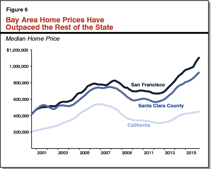
Bay Area Has Experienced Exceptional Growth in Prices and Rents. House prices and rents have increased significantly faster in the Bay Area than in the rest of the state. Figure 6 shows the 15–year trend of median home prices in San Francisco and in Santa Clara County, which includes San Jose. Median house prices in San Francisco ($1.1 million) and Santa Clara County ($926,000) grew by 15 percent and 13 percent, respectively, over the past year. Since 2011, house prices in these counties have grown by over 60 percent. Rents in San Francisco and Santa Clara similarly rose by over 30 percent between 2011 and 2014.
Building Remains Below Historical Levels Despite Price and Rent Growth. Residential building permits appear to be on pace to total roughly 98,000 in 2015, a notable increase over building levels in the prior two years (around 85,000 per year). Despite this increase, residential building remains below historical levels, as well as below what recent population growth would suggest. During the 2000s, building permits averaged 146,000 units per year. Our main scenario assumes permits will continue to climb over the next few years, but remain below historical levels. It is not entirely clear why building has not returned to historical levels. Several factors, however, likely play some role. Data suggests that household formations—for example, when younger people move out of parents’ homes—have fallen in recent years. As discussed in our March 2015 report, California’s High Housing Costs: Causes and Consequences, it is also possible that local government resistance to building is preventing developers from increasing production of new housing. Some reports also suggest that builders are experiencing labor shortages in certain markets.
Pluses and Minuses for Government Budgets and Economy. Recent growth in house prices and rents has contributed to robust growth in state and local revenues—particularly property taxes. Statewide assessed property values increased by 6 percent in both 2014–15 and 2015–16, compared to an average annual rate of less than 0.5 percent over the preceding five years. We anticipate this robust growth to continue in the near term, with assessed values projected to grow by just over 6 percent in 2016–17.
Nonetheless, high house prices and rents present some risks to the state’s economy. Rising housing costs force Californians to spend more of their income on housing, leaving less available for other purchases. High housing costs also can deter workers from moving to the state’s most productive regions—where housing costs tend to be the highest—constraining business recruitment and expansion. In the long term, future growth in the economy and state and local revenues could be dampened if new housing production continues to fall short of demand.
Revenues
Figure 7 summarizes our main scenario revenue outlook for California’s General Fund through 2019–20. Figure 8 shows how our key revenue numbers differ from June 2015 state budget assumptions (which were based on the Governor’s May 2015 revenue estimates). Below, we discuss some key issues concerning (1) the personal income tax (PIT), which generates about two–thirds of General Fund revenues, and (2) the state’s other key taxes.
Figure 7
LAO Revenue Summary: November 2015 Main Scenario
General Fund and Education Protection Account Combined (Dollars in Millions)
|
2014–15 |
2015–16 |
2016–17 |
2017–18 |
2018–19 |
2019–20 |
|
|
Personal income tax |
$76,400 |
$81,676 |
$84,274 |
$88,946 |
$90,057 |
$91,122 |
|
Sales and use tax |
23,709 |
24,971 |
25,351 |
25,980 |
26,808 |
28,091 |
|
Corporation tax |
9,714 |
10,198 |
10,685 |
10,842 |
11,089 |
11,557 |
|
Subtotal, “Big Three” Revenues |
($109,823) |
($116,844) |
($120,311) |
($125,768) |
($127,953) |
($130,770) |
|
Percent growth from prior year |
11.8% |
6.4% |
3.0% |
4.5% |
1.7% |
2.2% |
|
Insurance tax |
$2,444 |
$2,493 |
$2,582 |
$2,682 |
$2,796 |
$2,903 |
|
Other revenues |
1,993 |
2,094 |
1,727 |
1,889 |
1,990 |
2,090 |
|
Transfers to Budget Stabilization Account |
–1,606 |
–4,035 |
–1,593 |
–1,550 |
–1,368 |
–1,016 |
|
Other net transfers in (out)a |
–409 |
–1,082 |
156 |
0 |
–34 |
–257 |
|
Total Revenues and Transfers |
$112,244 |
$116,315 |
$123,183 |
$128,789 |
$131,337 |
$134,490 |
|
Proposition 2 Inputs |
||||||
|
Taxes on capital gains |
N/A |
$13,940 |
$12,488 |
$12,604 |
$11,990 |
$10,557 |
|
As percent of General Fund taxes |
N/A |
11.6% |
10.1% |
9.7% |
9.1% |
7.8% |
|
aFor 2016–17 through 2019–20 (unlike prior fiscal years), no special fund loan repayments are included in this line as transfers out. To the extent those repayments are to be made in future years, they are assumed to occur as Proposition 2 debt payment expenditures. |
||||||
Personal Income Tax
Our main scenario PIT estimates continue to be higher than the administration’s projections from earlier this year, as summarized in Figure 8.
Figure 8
Comparing Key LAO and Administration Revenue Numbers
General Fund and Education Protection Account Combined (In Millions)
|
2014–15 |
2015–16 |
2016–17 |
|||||||||
|
LAO Nov. 2015 |
Admin. June 2015 |
Change |
LAO Nov. 2015 |
Admin. June 2015 |
Change |
LAO Nov. 2015 |
Admin. June 2015 |
Change |
|||
|
Personal income tax |
$76,400 |
$75,384 |
$1,016 |
$81,676 |
$77,700 |
$3,976 |
$84,274 |
$81,652 |
$2,623 |
||
|
Sales and use tax |
23,709 |
23,684 |
25 |
24,971 |
25,240 |
–269 |
25,351 |
25,761 |
–410 |
||
|
Corporation tax |
9,714 |
9,809 |
–94 |
10,198 |
10,342 |
–144 |
10,685 |
11,073 |
–388 |
||
|
“Big Three” Revenues |
$109,823 |
$108,877 |
$946 |
$116,844 |
$113,281 |
$3,564 |
$120,311 |
$118,485 |
$1,825 |
||
Historical Growth Patterns. The PIT generally is the key revenue source to consider when thinking about the prospects for state revenue growth. We estimate that the PIT grew by an extraordinary 14 percent in 2014–15, with an additional 7 percent increase now expected for 2015–16. Since 2000–01, the annual growth of PIT has, on average, been about 5 percent. (This calculation includes some tax policy changes that have occurred, as well as two recessions.) PIT growth has exceeded 5 percent in eight fiscal years since 2000–01 and fallen short of that threshold in seven years. Those seven years include ones affected by (1) the bust of the dot.com stock bubble in the early 2000s, (2) the bust of the housing bubble in the mid–2000s and the subsequent recession, and (3) the decline in taxable income in 2013 (associated with the federal “fiscal cliff”) when high–income taxpayers accelerated financial transactions to 2012 in order to avoid later federal tax increases. Accordingly, in a year unaffected by an income tax cut, an economic slowdown, or a stock market drop, the state’s elected leaders reasonably can expect something like 5 percent (or more) PIT growth.
Slow Growth Assumed for 2016–17. Our main scenario anticipates slower PIT growth in 2016–17—only 3.2 percent. The key underlying reason for the slow growth rate in our 2016–17 PIT estimate is our assumption about stock prices. Specifically, we assume that the average closing price of the S&P 500 stock index during the current quarter will be 1,993—below the 2,100 level posted for much of early 2015. This level was consistent with the S&P 500 index as of October 14, when we were finalizing our main scenario assumptions. With the price–to–earnings ratio of the S&P 500 now above 20—somewhat high historically, but below some prior “bubble” periods—we assume very slow future growth of stock prices, consistent with our practices in recent years. Under our main scenario, therefore, the S&P 500 does not return to the 2,100 level until the middle of 2017. This causes our estimate of net capital gains income on California resident tax returns to fall from around $150 billion in 2015 to around $130 billion in each of the next three years. That drop in capital gains—resulting from our S&P 500 stock price assumption—causes our slow estimated PIT growth rate for 2016–17.
The assumed trend for wage income offsets somewhat the impact of our capital gains assumptions. Wages make up the large majority of taxable income, and our main scenario assumes robust growth in wages and salaries reported on California PIT returns of about 7 percent per year in 2016 and 2017.
It is impossible to predict future stock and capital gains growth and difficult to precisely project wage growth. Therefore, actual PIT results in 2016–17 (and even 2015–16) could result in revenues being billions of dollars above or below our main scenario estimates. Yet, in fulfilling its constitutional responsibility to determine a state revenue estimate annually for the budget, the Legislature must make assumptions about wages and uncertain stock prices and capital gains taxes.
Scheduled Expiration of Proposition 30. Proposition 30’s temporary PIT rate increases on the highest–income Californians expire at the end of 2018. As a result, 2018–19 essentially reflects a half year of those revenues in our main scenario, and 2019–20 includes no Proposition 30 PIT revenues. (The scheduled expiration of Proposition 30’s sales tax rate increase slows anticipated revenue growth in 2016–17 and 2017–18, as discussed below.) In this main scenario, with continuing economic growth, there continues to be no “cliff effect” as Proposition 30 revenues end. The expiration of Proposition 30 slows, but does not stop, PIT growth in our main scenario. If, however, an economic slowdown were to occur around 2019, the fall off of Proposition 30 revenues would exacerbate any slowdown or decline in PIT revenues.
As this publication was being drafted, initiative proposals to extend Proposition 30’s PIT increases were being introduced. This publication’s scenarios, however, all assume that Proposition 30 expires because that is the tax policy in current state law.
Other Key Taxes
While legislative discussions about revenue estimates recently have focused on the PIT, the two other key state taxes—the sales and use tax (SUT) and the corporation tax (CT)—together make up around one–third of General Fund revenues. As such, the SUT and CT also play important roles in determining the state’s annual revenue estimate.
Sales and Use Taxes. Estimated General Fund SUT revenue totaled $23.7 billion in 2014–15, $25 million higher than the amount assumed in the state’s 2015–16 budget plan. In our main scenario, SUT revenues grow to $25.0 billion in 2015–16, about $270 million lower than the assumption in the 2015–16 budget. Under this scenario, SUT revenues then grow more slowly as the one–quarter cent Proposition 30 SUT increase ends in December 2016. This results in slower General Fund SUT growth—around 2 percent per year—over the next two fiscal years, with this revenue source totaling an estimated $25.4 billion in 2016–17 and $26.0 billion in 2017–18.
Starting in 2014–15, certain sales of manufacturing or research and development equipment became exempt from the General Fund portion of the SUT. The administration initially projected that the new exemption would reduce General Fund revenue by $486 million in 2014–15 and by more than $500 million in subsequent years. The administration’s current estimate for 2014–15 is $128 million—about one–quarter of the amount initially projected. Our main scenario assumes that this amount grows to slightly less than $200 million per year in 2015–16 and 2016–17.
Corporation Taxes. While CT revenues have steadily grown since the 2011–12 fiscal year, the 2015–16 budget plan appears to have overestimated CT revenues in 2014–15 and, we expect, in 2015–16 as well. CT revenues totaled an estimated $9.7 billion in 2014–15, about $100 million less than the budget assumption. This was due largely to several hundred million dollars in refund settlements over the past several months. (Under the state’s complicated process for accruing, or assigning, revenues to specific fiscal years, these refunds generally are accrued to prior fiscal years.) While the refunds were not entirely unexpected, it is very difficult to predict their timing. In our main scenario, CT revenues are projected to total $10.2 billion in 2015–16, about $150 million below the 2015–16 budget assumption. That discrepancy, however, is relatively small, and estimated year–to–year growth in CT revenues currently reflects a fairly healthy and growing economy.
Corporate profits and CT revenue have both grown rapidly since the last recession. Our main scenario assumes that the rate of growth in corporate profits will slow considerably for several years beginning in 2017. This causes estimated CT revenue to grow relatively slowly after 2016–17, but these growth trends may differ substantially from actual results for a variety of reasons. In particular, there are many factors that determine the total amount of CT revenue in any year, including the use of tax deductions and tax credits. Two tax provisions in particular can have an enormous effect on final tax collections: net operating loss deductions and research tax credits. Each of these reduces aggregate tax liabilities by more than $1 billion per year. Corporations’ use of these provisions in any given year is highly uncertain and highly variable, and each can increase or reduce CT revenue from one year to another by hundreds of millions of dollars.
Litigation. There are always major revenue–related lawsuits and tax agency proceedings that affect state revenues. At the time this report was prepared, the state was awaiting an upcoming state Supreme Court decision concerning the apportionment of income between states by multi–state corporations. If the state loses that lawsuit, its potential liability could be hundreds of millions of dollars or more. (A recent state disclosure to bond investors said the potential exposure to refund claims in this case could exceed $750 million.) On the other hand, a recent appellate opinion could require health plans (such as Blue Shield and Anthem Blue Cross) to start paying the state’s insurance tax, with some net revenue gain possible for the General Fund. In cases like these, it is difficult to know how soon revenue gains or losses will materialize for the state. Large tax cases tend to result in long appeals and multiple proceedings spread out over many years. Our main scenario assumes no changes to state revenue due to these or other ongoing lawsuits and tax agency proceedings.
Chapter 3: Spending Outlook
Main Scenario Estimates Reflect Economic Assumptions. Figure 1 displays our main scenario spending estimates through 2019–20. Our main scenario assumes that current spending laws and policies are not changed and that the economy grows steadily throughout the period. Should the economy fall into recession in the next few years, or if the economic growth pattern differs from our assumptions, spending in many programs could be very different. For example, state spending on Proposition 98 education programs depends on changes in personal income (a broad measure of the economy), local property taxes, and state General Fund revenues. Because we cannot precisely “predict” how these factors will change, Proposition 98 spending in the future could be quite different from that shown in the figure.
Figure 1
General Fund Spending Under LAO Main Scenario
Includes Education Protection Account (Dollars in Millions)
|
Estimates |
Outlook |
Average Annual Growtha |
||||||
|
2014–15 |
2015–16 |
2016–17 |
2017–18 |
2018–19 |
2019–20 |
|||
|
Education Programs |
||||||||
|
Proposition 98b |
$50,497 |
$49,444 |
$50,213 |
$52,110 |
$52,376 |
$52,992 |
1.7% |
|
|
UC |
2,991 |
3,136 |
3,261 |
3,391 |
3,527 |
3,668 |
4.0 |
|
|
CSU |
2,763 |
2,988 |
3,121 |
3,257 |
3,393 |
3,534 |
4.3 |
|
|
Student Aid Commission |
1,527 |
1,614 |
1,786 |
1,935 |
2,045 |
2,160 |
7.6 |
|
|
Child carec |
822 |
942 |
950 |
965 |
984 |
1,005 |
1.7 |
|
|
Health and Human Services |
||||||||
|
Medi–Cal |
17,521 |
17,993 |
20,504 |
20,915 |
22,567 |
24,133 |
7.6 |
|
|
CalWORKs |
619 |
588 |
266 |
178 |
135 |
127 |
–31.9 |
|
|
SSI/SSP |
2,790 |
2,811 |
2,846 |
2,883 |
2,920 |
2,958 |
1.3 |
|
|
IHSS |
2,193 |
2,802 |
2,788 |
2,883 |
3,008 |
3,140 |
2.9 |
|
|
DDS |
3,130 |
3,496 |
3,550 |
3,651 |
3,760 |
3,920 |
2.9 |
|
|
DSH |
1,498 |
1,537 |
1,542 |
1,546 |
1,551 |
1,551 |
0.2 |
|
|
Other major programsd |
1,997 |
2,173 |
2,159 |
2,168 |
2,184 |
2,199 |
0.3 |
|
|
CDCR |
9,499 |
9,530 |
9,500 |
9,523 |
9,549 |
9,568 |
0.1 |
|
|
Judiciary |
1,409 |
1,511 |
1,515 |
1,548 |
1,580 |
1,613 |
1.7 |
|
|
CalSTRS |
1,486 |
1,935 |
2,468 |
1,728 |
1,674 |
1,679 |
–3.5 |
|
|
Infrastructure Debt Servicee |
5,250 |
5,353 |
5,602 |
5,524 |
6,083 |
6,041 |
3.1 |
|
|
Proposition 2 Debt Paymentsf |
— |
227 |
1,593 |
1,550 |
1,368 |
1,016 |
— |
|
|
Other Programs |
9,347 |
7,183 |
7,454 |
8,048 |
8,642 |
9,272 |
6.6 |
|
|
Totals |
$115,340 |
$115,262 |
$121,119 |
$123,804 |
$127,345 |
$130,575 |
3.2% |
|
|
Percent change |
— |
–0.1% |
5.1% |
2.2% |
2.9% |
2.5% |
— |
|
|
aFrom 2015–16 to 2019–20. bReflects the General Fund component of the Proposition 98 minimum guarantee. Average annual growth in the minimum guarantee—the General Fund and local property tax revenue combined—is 2.9 percent over the period. c Stage 1 child care costs included in CalWORKs. A portion of State Preschool costs is reflected in Proposition 98. d Includes DHCS family health and state operations, DPH, DCSS, and DSS programs not itemized above. Smaller health and human services programs are included in “other programs.” eDebt service on general obligation and lease–revenue bonds generally used for infrastructure. Does not include: (1) lease–revenue debt service for community colleges, which is included under Proposition 98, or (2) UC’s and CSU’s debt service, which is included in their respective line items. fFor 2015–16, includes $96 million UC pension payment, $84 million loan repayment to the Transportation Investment Fund, and $47 million in interest on special fund loans. Other Proposition 2 debt payments in 2015–16 are reflected in revenues and transfers. Beginning in 2016–17, reflects our estimate of debt payments required under Proposition 2. The Legislature could choose to spend these amounts on additional special fund loan repayments, Proposition 98 “settle–up,” or paying down unfunded liabilities for pension and retiree health benefits. IHSS = In–Home Supportive Services; DDS = Department of Developmental Services; DSH = Department of State Hospitals; DHCS = Department of Health Care Services; DPH = Department of Public Health; DCSS = Department of Child Support Services; and DSS = Department of Social Services. |
||||||||
Moderate Spending Growth Under This Scenario. Under our main scenario, General Fund spending increases over the period at an average annual rate of 3.2 percent. Two key programs—Proposition 98 and Medi–Cal—experience very different growth patterns. General Fund spending on Proposition 98 programs grows slowly over the period at an average annual rate of 1.7 percent, largely due to two factors. First, the gradual expiration of Proposition 30’s temporary taxes slows General Fund revenue growth over four fiscal years. Second, healthy growth in local property taxes offset state spending on Proposition 98. On the other hand, our main scenario reflects 7.6 percent average annual growth on Medi–Cal, the second largest General Fund program. The growth patterns in these two key programs explain the moderate General Fund spending growth reflected in our main scenario.
Education
Education Spending. In this section, we focus on Proposition 98, the universities, student financial aid programs, and child care programs. The Proposition 98 section estimates combined spending for a large portion of the state’s subsidized preschool program, elementary and secondary education (commonly referred to as K–12 education), and the California Community Colleges. The next section estimates spending for the University of California and the California State University. The financial aid section estimates spending for the Cal Grant program, Middle Class Scholarships, and a few small specialized programs. The last section estimates spending for the rest of the state’s preschool program as well as child care programs.
Proposition 98
Proposition 98 Minimum Guarantee for Schools and Community Colleges. State budgeting for schools and community colleges is governed largely by Proposition 98, passed by voters in 1988. The measure, modified by Proposition 111 in 1990, establishes a minimum funding requirement, commonly referred to as the minimum guarantee. Both state General Fund and local property tax revenue apply toward meeting the minimum guarantee. In addition to Proposition 98 funding, schools and community colleges receive funding from the federal government, other state sources (such as the lottery), and various local sources (such as parcel taxes).
Calculating the Minimum Funding Guarantee. The Proposition 98 minimum guarantee is determined by one of three tests set forth in the State Constitution (see Figure 2). These tests depend upon several inputs, including changes in K–12 average daily attendance (ADA), per capita personal income, and per capita General Fund revenue. Though the calculation of the minimum guarantee is formula–driven, a supermajority of the Legislature can vote to suspend the formulas and provide less funding than they require. This happened in 2004–05 and 2010–11. In some cases, including as a result of a suspension, the state creates an out–year obligation referred to as a “maintenance factor.” The state is required to make maintenance factor payments when year–to–year growth in state General Fund revenue is relatively strong. Though in most years the state has provided an amount at or close to the minimum guarantee, the state has discretion to provide any amount above the minimum guarantee.
Figure 2
Constitution Sets Forth Three Tests for Calculating Proposition 98 Minimum Guarantee
|
Test 1—Share of General Fund. Ensures Proposition 98 programs receive at least 40 percent of state General Fund revenue. This test applies only when it results in a higher funding level than Test 2 or Test 3. Test 1 has been operative 4 of the last 27 years. |
|
Test 2—Growth in Personal Income. Adjusts prior–year Proposition 98 funding for changes in K–12 attendance and per capita personal income. This test applies when higher than Test 1 but lower than Test 3. Test 2 has been operative 14 of the last 27 years. |
|
Test 3—Growth in General Fund Revenue. Adjusts prior–year Proposition 98 funding for changes in K–12 attendance and per capita General Fund revenue. This test applies when higher than Test 1 but lower than Test 2. Test 3 has been operative 7 of the last 27 years. |
|
Note: In 2 of the last 27 years, the state suspended Proposition 98. |
2014–15 and 2015–16 Updates
2014–15 Minimum Guarantee Up $1.3 Billion From Budget Act Estimate. Of this amount, $889 million is covered by state General Fund and $409 million by higher local property tax revenue. Test 1 remains the operative test in 2014–15. Test 1, when coupled with maintenance factor application, results in the minimum guarantee going up virtually dollar for dollar with increases in General Fund revenue. As shown in Figure 3, the $904 million increase in applicable state General Fund revenue increases the minimum guarantee by $889 million. Part of this increase results from a higher required maintenance factor payment ($541 million). The remainder of the increase in the guarantee is due to an upward revision in local property tax estimates. A portion of the property tax revision ($243 million) is due to an increase in the amount of ongoing revenue shifted to schools and community colleges from the dissolution of redevelopment agencies. (The state dissolved these agencies in 2011 and provided for a gradual shift of their revenue to schools and other local governments as their debts are retired.) Higher–than–expected collections from several smaller components of property tax revenue account for the remainder of the increase. Although local property tax revenue normally offsets the General Fund share of Proposition 98 funding, Test 1 years are exceptions, with Proposition 98 funding increasing with increases in local revenue.
Figure 3
Updating Estimates of 2014–15 and 2015–16 Minimum Guarantees
(Dollars in Millions)
|
2014–15 |
2015–16 |
||||||
|
2015–16 Budget Plan |
November LAO Estimate |
Change |
2015–16 Budget Plan |
November LAO Forecast |
Change |
||
|
Minimum Guarantee |
|||||||
|
General Fund |
$49,608 |
$50,497 |
$889 |
$49,416 |
$49,444 |
$27 |
|
|
Local property tax |
16,695 |
17,104 |
409 |
18,993 |
19,704 |
711 |
|
|
Totals |
$66,303 |
$67,601 |
$1,298 |
$68,409 |
$69,148 |
$739 |
|
|
Key Information |
|||||||
|
General Fund tax revenuea |
$112,068 |
$112,972 |
$904 |
$116,619 |
$120,119 |
$3,500 |
|
|
K–12 average daily attendance |
5,994,522 |
5,981,073 |
–13,449 |
5,995,889 |
5,974,494 |
–21,395 |
|
|
Operative test |
1 |
1 |
— |
3 |
2 |
— |
|
|
Maintenance factor paid |
$5,402 |
$5,942 |
$541 |
— |
$195 |
$195 |
|
|
aReflects General Fund revenue that counts toward the Proposition 98 calculation. |
|||||||
Spike Protection Results in Smaller Increase to Ongoing Funding Level. In most years, Proposition 98 funding builds upon the level provided in the prior year. This dynamic means that increases in the guarantee in one year usually carry forward and result in a comparable increase the next year. In 2014–15, however, only the increase associated with the maintenance factor payment carries forward into 2015–16. The remaining increase is excluded due to a provision in the State Constitution known as spike protection. This is intended to prevent very large one–time spikes in revenue from increasing the guarantee to an unsustainably high level moving forward. Since its adoption in 1990, spike protection has been applied to the guarantee twice (in 2012–13 and 2014–15).
2015–16 Minimum Guarantee Up $739 Million From Budget Act Estimate. Two main factors account for this increase. First, the $541 million maintenance factor payment from 2014–15 carries forward, increasing the 2015–16 guarantee by a similar amount. Second, we estimate that General Fund revenue is up $3.5 billion compared with the budget plan estimate. With Test 2 projected to be operative, the guarantee is determined largely by growth in per capita personal income and is not directly affected by changes in General Fund revenue. The additional revenue does, however, require the state to make a $195 million maintenance factor payment. Upon making this payment, the state will have eliminated its entire maintenance factor obligation, ending the year with no maintenance factor outstanding for the first time since 2005–06.
Further Changes in Revenue Would Have Little Effect on 2015–16 Guarantee. In 2015–16, the guarantee is relatively insensitive to changes in revenue. Under our main scenario, with Test 2 the operative test and no further maintenance factor payments required, the 2015–16 guarantee no longer depends directly on growth in state revenue. We estimate that General Fund revenue could increase by as much as $8 billion above our projections with no corresponding increase in the guarantee. Conversely, General Fund revenue could fall below our projections by as much as $4 billion with the only Proposition 98 effect being that the state no longer would be required to make the remaining $195 million maintenance factor payment in 2015–16. This dynamic contrasts notably with the situation in 2014–15, under which the guarantee changes nearly dollar for dollar with any change in state General Fund revenue.
Virtually All $739 Million Increase Covered With Higher Property Tax Revenue. Though the 2015–16 guarantee is up $739 million, the General Fund share of the guarantee is up only $27 million. Increases in local property tax revenue cover the remaining $711 million increase. About half of this amount ($334 million) is due to higher–than–expected ongoing revenue from the dissolution of redevelopment agencies. The remainder is due primarily to higher assessed property values. Whereas the budget plan assumed assessed values would grow statewide by 5.5 percent, the latest available data from county assessors indicates that the increase will be about 6 percent.
Drop in K–12 ADA Frees Up Some Funding Within Guarantee. Compared to budget act assumptions, we estimate K–12 ADA has fallen by about 13,000 in 2014–15 and by about 21,000 in 2015–16. Due to a two–year hold harmless provision in the State Constitution, these ADA declines do not affect the guarantees in 2014–15 and 2015–16. The ADA drops, however, reduce the cost of many educational programs, including the Local Control Funding Formula (LCFF), thereby freeing up roughly $300 million across the two years for other Proposition 98 priorities.
About $2.3 Billion Available for One–Time Purposes. For 2014–15 and 2015–16 combined, the minimum guarantee has increased a total of $2 billion (see Figure 3). Given the 2014–15 fiscal year is already over and districts are well into their 2015–16 fiscal year, this additional funding in practical terms is available for one–time purposes. Combined with the $300 million in ADA–related savings from 2014–15 and 2015–16, the state has about $2.3 billion to allocate for its one–time priorities. Over the past few years, the state has used one–time funding to support a range of activities including (1) implementation of the Common Core State Standards, (2) career technical education, (3) teacher training and support, and (4) paying down several outstanding K–14 obligations. As of the 2015–16 budget plan, the state had retired some of these latter outstanding obligations but had not entirely paid down the K–14 mandates backlog. In recent years, the state has reduced the K–14 mandates backlog considerably (by more than $4 billion), but we estimate the state still has an unaudited backlog of about $2 billion ($1.7 billion for schools and $300 million for community colleges).
2016–17 Budget Planning
2016–17 Guarantee $2.3 Billion Higher Than Revised 2015–16 Guarantee. We project the minimum guarantee will grow from $69.1 billion in 2015–16 to $71.4 billion in 2016–17, an increase of $2.3 billion (3.3 percent). Test 3 is operative, with the change in the guarantee driven primarily by projected growth in per capita General Fund revenue. Other factors affecting the guarantee include a slight decline in K–12 attendance (0.3 percent) and the requirement for the state to make a $618 million supplemental payment. (A state law requires a supplemental payment whenever Test 3 is operative and Proposition 98 funding would otherwise grow less quickly than the rest of the state budget.) Given the guarantee is still growing more slowly than our projected 5.3 percent growth in per capita personal income, the state creates a $1.1 billion maintenance factor obligation.
Two–Thirds of Increase Covered With Higher Local Property Tax Revenue. Of the $2.3 billion increase in the 2016–17 guarantee, the General Fund share is $770 million. A $1.5 billion increase in local property tax revenue covers the remainder of the increase in the guarantee, with local property tax revenue up 7.8 percent over the 2015–16 level. Two main factors account for this increase:
- Assessed Property Values Projected to Grow at Relatively Strong Rate. We project assessed values will increase by 6.3 percent in 2016–17, largely reflecting the strong recovery in the housing market that has occurred over the past several years. This growth rate equates to a $1.1 billion increase in local property tax revenue for schools and community colleges.
- Final Shift of Revenue From End of “Triple Flip.” The triple flip is phasing out during the 2015–16 fiscal year, with the associated local property tax revenue beginning to flow back to schools and community colleges. The total revenue involved is about $1.6 billion on an ongoing basis. Schools and community colleges will receive $1.2 billion of this amount in 2015–16 and the remainder (about $400 million) in 2016–17. (The triple flip was a complex financing mechanism under which the state diverted local sales tax revenue to pay off certain state bonds, backfilled cities and counties with property tax revenue, and backfilled schools and community colleges with state General Fund.)
$3.6 Billion Available for Proposition 98 Priorities in 2016–17 Under Main Scenario. As shown in Figure 4, the 2015–16 Budget Act included $68.4 billion in spending to meet the minimum guarantee (as estimated at that time). Of this amount, $67.9 billion was ongoing spending and $551 million was one–time spending. Given projected growth in the 2016–17 guarantee to $71.4 billion, the state has $3.6 billion available for its 2016–17 Proposition 98 priorities.
Figure 4
$3.6 Billion Increase in Proposition 98 Funding Projected for 2016–17
LAO Main Scenario (In Millions)
|
2015–16 Budget Act Spending Level |
$68,409 |
|
Back out one–time actions: |
|
|
Secondary school career technical education grantsa |
–$250 |
|
CCC mandate backlog |
–117 |
|
CCC maintenance and instructional equipment |
–100 |
|
K–12 Internet infrastructure grants |
–50 |
|
K–12 mandate backlog |
–31 |
|
CCC Cal Grant B administration |
–3 |
|
Total One–Time Actions |
–$551 |
|
2015–16 Ongoing Spending |
$67,858 |
|
Annualize preschool slotsb |
$31 |
|
New Funds Available in 2016–17c |
$3,558 |
|
2016–17 Minimum Guarantee |
$71,447 |
|
a In 2015–16, this program received an additional $150 million from one–time funds. b Funded beginning January 1, 2016. c The state has committed to spend $300 million in 2016–17 for the second year of the secondary school career technical education grants. The state could cover this cost using any available Proposition 98 funding from any fiscal year. |
|
2016–17 Guarantee Is Somewhat Sensitive to Changes in State General Fund Revenue. Whereas the 2014–15 guarantee was highly sensitive to changes in state General Fund revenue and the 2015–16 guarantee is highly insensitive to changes, the 2016–17 guarantee is moderately sensitive. Relative to our main scenario, a $1 increase or decrease in General Fund revenue in 2016–17 would cause a corresponding increase or decrease in the guarantee of about 50 cents. If General Fund revenue were to increase by $2 billion above our main scenario, the guarantee would increase by about $1 billion. (If revenue were to increase beyond this level, however, the guarantee would be unlikely to increase further. This is because Test 2 would become operative, with the guarantee then linked to per capita personal income rather than state revenue.) If General Fund revenue were to decline by $5 billion from our main scenario, the guarantee would decline by about $2.5 billion, dropping below the prior–year funding level.
In Past Several Years, State Has Minimized Risk by Designating Some Funding for One–Time Activities. Given the difficulty of predicting recessions, stock market slowdowns, and other events that can reduce General Fund revenue, the state over the past few years has dedicated some available Proposition 98 funding to one–time activities. If the guarantee falls below projections, the expiration of prior–year, one–time funding provides a buffer, reducing the likelihood of potential cuts to ongoing K–14 programs. Allocating a portion of available funding for one–time priorities would mitigate the effect of a decline in the guarantee from 2016–17 to 2017–18. For example, under the recession scenario we discuss in Chapter 4, General Fund revenue declines by nearly $8.5 billion (7 percent) from 2016–17 to 2017–18. (By comparison, during the last two recessions, the state experienced much larger year–over–year declines.) Under the recession scenario, the 2017–18 guarantee would experience a year–over–year decline of $4.6 billion. If the state were to designate some available 2016–17 funding for one–time activities, it would reduce the magnitude of potential reductions to ongoing programs in 2017–18.
Outlook for Later Years
Although both the Legislature and schools likely view near–term Proposition 98 issues as the most pressing, a number of significant issues unfold over the forecast period. Most notably, these issues include the phase out of the Proposition 30 taxes, the phase in of LCFF funding increases, and the cost pressures associated with increased contributions to the California State Teachers’ Retirement System (CalSTRS). Members of the Legislature also have asked whether a deposit in the state school reserve might occur in the coming years, thereby triggering the associated caps on school district reserve levels. Below, we describe the Proposition 98 outlook through 2019–20 under our main scenario and examine the above issues in more detail.
Under Main Scenario, Guarantee in 2019–20 More Than $8 Billion Higher Than 2015–16. Figure 5 shows our Proposition 98 projections under our main scenario from 2015–16 through 2019–20. As shown in the figure, Proposition 98 funding grows from $69.1 billion in 2015–16 to $77.5 billion in 2019–20, an annual average growth rate of 2.9 percent. General Fund costs grow more slowly, from $49.4 billion in 2015–16 to $53 billion in 2019–20. This slower growth in the General Fund share of Proposition 98 results from the relatively fast growth in local property tax revenue, which increases from $19.7 billion in 2015–16 to $24.5 billion in 2019–20. The average annual growth over the period is 1.7 percent for the General Fund and 5.6 percent for local property tax revenue.
Figure 5
Proposition 98 Outlook
LAO Main Scenario (Dollars in Billions)
|
2015–16 |
2016–17 |
2017–18 |
2018–19 |
2019–20 |
|
|
Minimum Guarantee |
|||||
|
General Fund |
$49.4 |
$50.2 |
$52.1 |
$52.4 |
$53.0 |
|
Local property tax |
19.7 |
21.2 |
22.5 |
23.4 |
24.5 |
|
Totals |
$69.1 |
$71.4 |
$74.6 |
$75.8 |
$77.5 |
|
Change From Prior Year |
|||||
|
Total guarantee |
$1.5 |
$2.3 |
$3.2 |
$1.2 |
$1.6 |
|
Percent change |
2.3% |
3.3% |
4.4% |
1.6% |
2.2% |
|
General Fund |
–$1.1 |
$0.8 |
$1.9 |
$0.3 |
$0.6 |
|
Percent change |
–2.1% |
1.6% |
3.8% |
0.5% |
1.2% |
|
Local property tax |
$2.6 |
$1.5 |
$1.3 |
$1.0 |
$1.0 |
|
Percent change |
15.2% |
7.8% |
5.9% |
4.3% |
4.4% |
|
Maintenance Factor |
|||||
|
Amount created (+)/paid (–) |
–$0.2 |
$1.1 |
$0.1 |
$2.6 |
$2.1 |
|
Total outstandinga |
— |
$1.1 |
$1.3 |
$4.0 |
$6.3 |
|
Operative Test |
2 |
3 |
3 |
3 |
3 |
|
Growth Rates |
|||||
|
K–12 average daily attendance |
–0.1% |
–0.3% |
–0.3% |
–0.5% |
–0.3% |
|
Per capita personal income (Test 2) |
3.8 |
5.3 |
4.9 |
5.6 |
5.3 |
|
Per capita General Fund (Test 3)b |
5.9 |
2.7 |
4.4 |
1.6 |
2.1 |
|
K–14 cost–of–living adjustment |
1.0 |
2.0 |
2.4 |
2.5 |
2.4 |
|
Assessed property values |
6.0 |
6.3 |
5.1 |
4.9 |
4.8 |
|
Public School System Stabilization Account Deposit? |
No |
No |
No |
No |
No |
|
aOutstanding maintenance factor grows each year with changes in K–12 attendance and per capita personal income. bAs set forth in the State Constitution, reflects change in per capita General Fund plus 0.5 percent. |
|||||
Growth in Local Property Tax Revenue Covers Majority of Proposition 98 Increase. As shown in Figure 5, property tax revenue grows throughout the period. As described earlier, the large increases unfolding in 2015–16 and 2016–17 are due primarily to the end of the triple flip. From 2017–18 through 2019–20, increases are due primarily to our projection that assessed property values—the main driver of growth in local property tax revenue—will grow by about 5 percent per year. Though this rate is somewhat below our projections for 2015–16 and 2016–17, it is comparable to historical averages. This growth equates to additional revenue of about $900 million per year. In addition, we project that revenue shifted from the former redevelopment agencies will increase by about $340 million in 2017–18 and by about $170 million per year in 2018–19 and 2019–20. (A portion of these increases, however, are offset by increases in excess taxes, the share of local revenue that does not count toward the minimum guarantee.)
Slower Growth in Guarantee as Proposition 30 Revenue Phases Out. As shown in Figure 5, the growth in the guarantee is relatively strong in the near term, with the guarantee projected to grow by 3.3 percent in 2016–17 and by 4.4 percent in 2017–18. These increases outpace the projected K–14 cost–of–living adjustment (COLA) in both of these years (projected at 2 percent and 2.4 percent, respectively). Growth in the guarantee slows toward the end of the period, with the guarantee projected to grow by 1.6 percent in 2018–19 and 2.2 percent in 2019–20. These increases are less than the projected K–14 COLA in both years (projected at 2.5 percent and 2.4 percent, respectively), meaning the state would have difficulty funding program expansions. The relatively low rate of growth in the guarantee in these years is due to the phase out of the income tax revenues associated with Proposition 30. Assuming the economy continues to expand, General Fund revenue and the minimum guarantee will continue to increase in those years, albeit at a relatively slow rate. (The sales tax portion of Proposition 30 phases out over the 2016–17 and 2017–18 fiscal years. The amount of revenue generated by the sales tax is relatively small compared with the income tax and has a smaller effect on the minimum guarantee.)
State Accumulates Increasingly Large Maintenance Factor Obligation Over Period. In our main scenario, strong growth in per capita personal income occurs over the period, with the annual increase exceeding 5 percent in three out of the four final years. When growth in per capita personal income exceeds growth in per capita General Fund revenue, Test 3 becomes the operative test for determining the minimum guarantee. Under our main scenario, Test 3 is operative from 2016–17 through 2019–20 and the state creates new maintenance factor each of these years. By 2019–20, the total amount of projected maintenance factor outstanding reaches $6.3 billion.
State Projected to Move Closer to Full LCFF Implementation by End of Period. In 2013–14, the state replaced most of its former school funding formulas with LCFF. In creating this new formula, the state set funding targets considerably higher than the 2012–13 funding levels and specified that the targets were to grow annually with the K–12 statutory COLA. Given the higher funding targets, the state phased in LCFF implementation, with full implementation expected in 2020–21. In 2013–14, LCFF was 72 percent funded. For 2015–16, we estimate LCFF is 90 percent funded. Under our main scenario, we estimate LCFF would be 96 percent funded by 2019–20 if the state dedicated increases in the minimum guarantee largely to LCFF. (Our estimate assumes the state creates no new categorical programs throughout the period but provides growth and COLA to most existing K–12 programs. We also assume community colleges receive 10.8 percent of the available Proposition 98 funding, consistent with their share of the guarantee under the 2015–16 budget plan.) Given the relatively high growth in the guarantee through 2017–18 and the relatively slow growth thereafter, virtually all of the progress toward LCFF implementation would occur by 2017–18.
CalSTRS Rate Increases Phasing In Over Period. State law ramps up school and community college districts’ CalSTRS contributions over the period. As scheduled in state law, district contribution rates increase from 10.7 percent of payroll in 2015–16 to 18.1 percent by 2019–20. Based on CalSTRS’ estimates, district costs will be nearly $3 billion higher in 2019–20 than 2015–16. Under our main scenario, the minimum guarantee grows more than $8 billion over the same period. Under the recession scenario we develop in Chapter 4 of this report, however, growth in the minimum guarantee would be less than the estimated increase in CalSTRS costs. (The final year of the CalSTRS increase is 2020–21—one year beyond the end of our forecast period—when district contributions will reach 19.1 percent of payroll.)
No Deposit Into Public School System Stabilization Account (PSSSA) Projected. Proposition 2, approved by voters in November 2014, created a new state reserve known as PSSSA. A related state law imposes a cap on school district reserves in the year after the state makes a deposit into the state reserve. Deposits are predicated on several conditions, including a requirement for the state to have paid off all maintenance factor created before 2014–15. Though we project this condition will be satisfied in 2015–16, we do not anticipate the state will meet the other conditions during the period. For example, a deposit requires the minimum guarantee to be growing more quickly than per capita personal income, but under our main scenario the guarantee would grow at a slower rate throughout the period. To meet all of the conditions in any year of the forecast period, the state very likely would need to experience a year–over–year revenue surge of at least several billion dollars relative to our projections. Absent such a surge, a deposit into the PSSSA would not occur and the local reserve cap would not take effect.
Universities
State Has Two Public University Systems. The University of California (UC) educates about 248,000 full–time equivalent undergraduate and graduate students at ten campuses. The California State University (CSU) educates about 378,000 full–time equivalent undergraduate and graduate students at 23 campuses. (These counts include resident and nonresident students.) Both university systems receive support for their core programs from a combination of state General Fund and student tuition revenue. In 2014–15, UC received $3 billion in state General Fund and $2.8 billion in student tuition revenue. That same year CSU received $2.8 billion in state General Fund and $2.1 billion in student tuition revenue.
Certain Components Excluded From Our University Forecast. We use UC’s and CSU’s main General Fund appropriation as a starting point for our forecast but back out the one–time $96 million payment provided in 2015–16 for UC’s outstanding pension liabilities. Our university forecast also does not include cost increases for CSU retiree health and pension contributions, as we forecast these as part of overall state employee costs. (The state only provides specific augmentations to cover pension rate adjustments relative to CSU’s 2013–14 payroll level, with CSU expected to cover any other pension cost increases from its base budget.) We also exclude one–time deferred maintenance funding for UC and CSU. (We display that funding in 2015–16 under “other programs” in Figure 1.) Lastly, we exclude Hastings College of the Law from our university forecast, as the state provides less than $15 million General Fund annually for the college. We combine Hastings College of the Law with other relatively small state programs and run one consolidated forecast for these programs.
Challenges in Running Current Law Forecast for UC and CSU. Whereas the State Constitution, state law, and federal law notably constrain some areas of the state budget (for example, K–14 education and health care), they do not notably constrain budgeting for UC and CSU. In any given year, the Legislature and the two university systems have significant discretion in deciding both what cost increases to fund and how to fund those increases (whether through the General Fund or tuition revenue).
Assumptions Underlying UC and CSU Forecast Based Largely on Current State Practice. Given these challenges, our university forecast relies primarily on current practice rather than current law. In some university budget areas, including general purpose base increases and certain lease–revenue payments, the state has acted somewhat consistently in recent years, such that past practice appears to be a reasonable indicator of future action. Though most of our assumptions are based on recent past practice, in a few areas—notably enrollment growth—we have had to use our judgment because the state’s recent actions have been somewhat inconsistent. For example, over the last ten years, the state has sometimes set enrollment expectations and funded associated growth, sometimes set enrollment expectations but required UC and CSU to fund the associated growth from base increases, and sometimes not set enrollment expectations but UC and CSU nonetheless increased enrollment. Below, we lay out our key forecast assumptions, and, when applicable, note any heightened degree of uncertainty surrounding an assumption.
Assume Base Increases for UC and CSU Through 2019–20. The state has provided general purpose base increases to UC and CSU in each of the last three years. In 2013–14 and 2014–15, UC and CSU received about the same size general purpose increases, whereas in 2015–16 they received notably different ongoing base increases. Because the Legislature has provided base increases the past few years, we assume that UC and CSU will continue to receive base increases from 2016–17 through 2019–20. Though state action regarding the size of these increases has not been entirely consistent the past three years, we assume UC and CSU receive the same dollar increases. Specifically, we calculate base augmentations for both university systems by increasing UC’s General Fund appropriation by 4 percent annually. We assume UC and CSU would cover increases in operational costs and most facility debt–service costs using these augmentations.
Assume Future Enrollment Growth Funded From Base Increases. As with other operational cost increases, we assume any enrollment growth beyond 2015–16 Budget Act expectations would be funded from base increases. This is consistent with state practice over the past three years. (For 2015–16, we assume both segments meet their enrollment growth expectations and UC receives the corresponding $25 million set forth in the budget act.) An upcoming freshman eligibility study, due to the Legislature in December 2016, may influence future budgetary decisions regarding enrollment. Until that study is released, estimating enrollment changes required to meet UC’s and CSU’s traditional eligibility pools is guesswork.
Assume Lease–Revenue Debt Payments to CSU. For 2016–17 and 2017–18, we assume CSU receives additional funding to cover projected increases in its lease–revenue debt service. This assumption is based on a previously agreed upon four–year schedule of increases, for which the Legislature has implemented the first two years of increases. For the last two years of the forecast period, we assume CSU covers all debt–service increases from within its base increases, consistent with our general debt–service assumption for both segments.
Assume No Tuition Increases. Over the last three years, the state General Fund has covered virtually all authorized UC and CSU cost increases. Moving forward, we assume the General Fund continues to bear the full cost, with no increase in student tuition levels. Under such a forecast, student tuition levels, already flat since 2011–12, would remain so through 2019–20 (nine consecutive years). This would be the longest period of flat tuition in many decades. Though it would be a particularly long period, extended tuition freezes are not entirely unprecedented. For example, the universities did not raise tuition from 1995–96 to 2001–02. Though we assume no increase in tuition under our main scenario, future decisions regarding tuition are uncertain. In some years past, the Legislature has raised tuition levels and General Fund support simultaneously whereas in other years it has raised tuition levels and reduced state funding. Such future decisions could impact university spending significantly.
Under LAO Outlook, University Spending Grows by $258 Million in 2016–17. Under our main forecast, UC General Fund spending grows to almost $3.3 billion from 2015–16 to 2016–17, an increase of $124 million (4 percent). Spending for CSU grows to $3.1 billion, an increase of $133 million (4.5 percent). Over the forecast period, UC and CSU spending continues to increase steadily, reaching $3.7 billion at UC and $3.5 billion at CSU in 2019–20. Given the various factors highlighted above, actual university spending in any given year could differ significantly from the amounts shown under our projections.
Financial Aid
The California Student Aid Commission (CSAC) is responsible for administering most state financial aid programs. The largest aid program CSAC administers is the Cal Grant program, which serves about 360,000 undergraduate students. This program primarily is funded with a combination of state General Fund and federal Temporary Assistance for Needy Families (TANF) monies. Other notable CSAC programs supported by the General Fund include Middle Class Scholarships and student loan assumption programs.
Key Assumptions for Forecast Period. For Cal Grants, we assume (1) annual participation growth of 5 percent; (2) the continued phase–in of awards for Dream Act students, with the program reaching full implementation in 2016–17; (3) the renewal of additional competitive awards (the state issued 3,250 additional new competitive awards in 2015–16); and (4) reductions in awards for students attending nonprofit colleges, with statutorily authorized reductions scheduled to take effect in 2017–18 and 2018–19. We also assume the state continues to use the same amount of federal TANF funds to offset a portion of General Fund Cal Grant costs. Additionally, we assume the continued phase–in of Middle Class Scholarship awards and the continued phase–out of all loan assumption programs. We assume no tuition increases at the universities. If tuition were raised during the forecast period, Cal Grants costs would be higher than reflected in Figure 1. For each 1 percent increase in tuition at UC and CSU, annual Cal Grant Costs would be $16 million higher.
Under Forecast, General Fund Financial Aid Costs Increase by $172 Million in 2016–17. Under our outlook, financial aid costs grow from $1.6 billion in 2015–16 to $1.8 billion in 2016–17—growth of $172 million (11 percent). Of this amount, $142 million reflects higher General Fund Cal Grant costs. Of the Cal Grant cost increases, $102 million reflects participation growth, $25 million is continued phase–in of Dream Act awards, and $14 million is higher renewal costs for competitive awards. In addition, we estimate cost increases of $34 million for Middle Class Scholarships and savings of $3.8 million for loan assumption programs.
Costs Over Period Very Sensitive to Assumption About Cal Grant Participation. Of the cost increases estimated for 2016–17, about 60 percent is attributable to assumed growth in Cal Grant participation. Over the rest of the period, our financial aid forecast remains very sensitive to assumptions about Cal Grant participation. Though we assume 5 percent annual growth based on a historical ten–year average, Cal Grant participation has risen even more quickly over the last three years, with an average annual growth rate of 10 percent. The recent rise in participation is due in part to efforts to increase the number of high schools electronically submitting grade point averages (GPAs) for all students. (Submitting a GPA is a requirement to apply for the Cal Grant high school entitlement award.) Additional factors likely are contributing to the increase, including continued improvements in outreach and administrative procedures at both the state and campus levels. If Cal Grant participation were to grow by 10 percent rather than 5 percent each year of the forecast period, annual financial aid costs in 2019–20 would be $2.7 billion rather than $2.2 billion.
Child Care
The state provides subsidized child care for families participating in California Work Opportunity and Responsibility to Kids (CalWORKs) and some other low–income, working families. Generally, CalWORKs families progress through three consecutive “stages” over the course of several years, with Stage 1 intended for families seeking employment, Stage 2 for families that have gained stable employment and are transferring off of cash assistance, and Stage 3 for families who have been off of cash assistance for at least two years. Our child care forecast includes expenditures for CalWORKs Stage 2 and Stage 3 care as well as non–CalWORKs care. We include Stage 1 costs in our CalWORKs forecast and a large portion of the State Preschool program in our Proposition 98 forecast.
Under Forecast, Child Care Costs Increase by Net of $8 Million in 2016–17. We project child care spending to increase from $942 million in 2015–16 to $950 million in 2016–17, an increase of less than 1 percent. The small increase in 2016–17 costs is the net result of several factors, including higher costs for annualizing rate and slot increases begun during 2015–16 and applying a 2 percent statutory COLA to non–CalWORKs programs. These higher costs are offset by the removal of prior–year, one–time funding as well as a small reduction reflecting a 0.5 percent decrease in the birth–to–four population in California. (State law specifies that non–CalWORKs child care programs be adjusted annually based on the change in this group.)
Child Care Costs Grow Steadily Throughout Remainder of Forecast Period. We project that annual child care costs will increase to about $1 billion by 2019–20. The bulk of this increase is due to our assumption that the state provides non–CalWORKs child care programs an annual statutory COLA. Over the period, the projected COLA rates range from a low of 2 percent in 2016–17 to a high of 2.5 percent in 2018–19. The average annual cost of the COLA is $17 million. (The birth–to–four population is projected to continue declining over the period, with the group 1 percent smaller in 2019–20 compared to 2016–17.)
California in Midst of Responding to New Federal Requirements. In addition to state General Fund, subsidized child care programs receive funding through the federal Child Care and Development Block Grant (CCDBG). In 2015–16, California received $573 million in CCDBG funding. The federal government reauthorized the CCDBG act in 2014—creating a new set of requirements for states. Most notably, the act changed how states are to set provider reimbursement rates, how frequently states are to inspect providers, and how much states must spend on activities designed to improve the quality of child care. The U.S. Department of Health and Human Services and states still are working out how to interpret and implement some of these new requirements. Decisions that (1) the federal government makes in developing associated regulations, (2) California makes in developing its required CCDBG state plan, and (3) the Legislature makes in implementing the new state plan all could have significant impact, affecting state costs and/or children served.
Health and Human Services
Overview of Health Services Provided. California’s major health programs provide health coverage and additional services for various groups of eligible persons—primarily poor families and children as well as seniors and persons with disabilities. The federal Medicaid program, known as Medi–Cal in California, is the largest state health program both in terms of funding and number of persons served. The Medi–Cal population has grown substantially since January 2014, reflecting an expansion of those eligible for Medi–Cal and a streamlining of eligibility requirements under the Patient Protection and Affordable Care Act (ACA), also known as federal health care reform. In addition, the state supports various public health programs. Although state departments oversee the management of these programs, the actual delivery of many services is carried out by counties and other local entities. Health programs are largely federally and state funded.
Overview of Human Services Provided. The state provides a variety of human services and benefits to its citizens. These include income maintenance for the aged, blind, and disabled; cash assistance and welfare–to–work services for low–income families with children; protection of children from abuse and neglect; the provision of home–care workers who assist the aged and disabled in remaining in their own homes; and community services and state–operated facilities for the mentally ill and developmentally disabled. Although state departments oversee the management of these programs, the actual delivery of many services is carried out by county welfare and child support offices, and other local entities. Most human services programs have a mixture of federal, state, and county funding.
Overall Spending Trends. The 2015–16 budget provides $31.7 billion in General Fund spending for health and human services (HHS) programs. We now estimate that these General Fund costs will be slightly lower—by a net of $150 million—in part reflecting lower caseloads than assumed by the budget for the CalWORKs population. Based on current law requirements, we project that General Fund spending for HHS programs will increase to $33.8 billion in 2016–17 and $34.4 billion in 2017–18. The significant growth in 2016–17 primarily reflects higher General Fund Medi–Cal spending, due mainly to the assumed repeal of the managed care organization tax as of 2016–17 and the inception of a state share of costs for the optional Medi–Cal expansion population under federal health care reform beginning in 2016–17. We assume that spending for HHS programs will eventually reach $38.2 billion in 2019–20 in our main economic scenario. Again, the bulk of the spending growth in the later years of the outlook reflect growth in Medi–Cal spending, due primarily to medical cost inflation and the increasing state share of costs for the optional Medi–Cal expansion population.
Although the average projected annual increase in HHS spending from 2015–16 through 2019–20 is about 5 percent, there is substantial variation in spending growth rates by program. For example, over these years, General Fund spending growth for Medi–Cal averages 7.6 percent per year, while the Supplemental Security Income/State Supplementary Program (SSI/SSP) is projected to grow modestly, with average annual growth of 1.3 percent. General Fund spending for the CalWORKs program is projected to substantially decline at an average annual rate of 32 percent, reflecting both projected caseload declines as well as the infusion of non–General Fund funding sources to support the program, as discussed further below.
Relatively Lower Caseload Growth in Some Programs Reduces Cost Pressures. The recession in the latter part of the 2000s raised unemployment and reduced income, resulting in historically high numbers of Californians enrolling in certain state HHS programs. As a result, caseload growth for several HHS programs from 2007–08 (the beginning of the recession) to 2011–12 (post–recession) was well above historical trends. Our main economic scenario assumes employment growth over the next four years, although at a slowing annual rate. Accordingly, our caseload projections for several HHS programs reflect substantially lower growth rates compared to the experience of the recent recessionary years, and in some cases—such as CalWORKs—we are anticipating caseload declines under our main economic scenario over some or all of the forecast period. This in turn reduces costs pressures.
Below, we discuss spending trends in the major HHS programs.
Medi–Cal
Overall Spending Trends. We estimate 2015–16 General Fund spending for Medi–Cal local assistance will be about $18 billion—0.3 percent (or $47 million) lower than what was assumed in the 2015–16 Budget Act. This mainly reflects lower spending on the Applied Behavioral Analysis benefit as a result of updated caseload and rate information. Our 2015–16 estimate also assumes that the President’s executive actions on immigration (discussed in more detail later in this report) will not be implemented. General Fund support increases 14 percent to $20.5 billion in 2016–17, largely as a result of underlying program growth and the loss of savings associated with the managed care organization (MCO) tax, which is assumed to expire without replacement at the end of 2015–16. Over the period of our outlook, other significant spending drivers include underlying program growth in caseload and per–enrollee costs, higher costs associated with the newly eligible population under the ACA (the so–called “optional expansion” population), and a decrease in federal funding for the Children’s Health Insurance Program (CHIP).
Caseload Has Continued to Climb Steeply. In June 2015—the most recent month for which enrollment counts may be considered nearly complete—total Medi–Cal caseload was over 12.6 million. This includes over 3 million individuals who became newly eligible for Medi–Cal under the optional ACA expansion. Total enrollment in June 2015 represents a net increase of roughly 1.3 million (or 11 percent) from total enrollment in June 2014. This is significant year–over–year growth, and may in part reflect a sustained boost in Medi–Cal uptake and retention under the ACA (such as enrollment simplification and outreach).
Delayed Redeterminations Likely Explains Some of Growth . . . We believe a major factor behind the persistent rise in caseload are ongoing delays and restrictions in the ability of counties to process and, when appropriate, terminate eligibility for many Medi–Cal enrollees during their annual redetermination. As an example, from January 2014 through June 2015, certain segments of the families and children population grew between 3 percent and 4 percent monthly. These same segments grew at similar rates annually between 2010–11 and 2012–13 (the period of sluggish economic recovery leading up to ACA implementation). We suspect the present high growth rates are partly the result of many enrollees failing to exit the program—even as their incomes rise above maximum eligibility thresholds—while new individuals continue to enter the rolls each month. Our communications with counties suggest their caseworkers continue to face significant barriers to completing redeterminations on a timely basis. These include technical challenges with the state’s new automation system for Medi–Cal eligibility and current litigation that blocks the state from terminating coverage for many individuals who fail to respond to the annual redetermination. In most cases, counties experiencing delays in redeterminations are required to grant continued eligibility for enrollees during the interim.
. . . Which Outlook Assumes Will Be Resolved in 2016–17. Our outlook assumes a large portion of 2015 redeterminations have not yet occurred for the optional expansion population, nor for those subgroups of families caseload that continue to exhibit uncharacteristic rapid growth. We further assume counties, beginning January 2016, will be able to process all pending redeterminations on their proper monthly schedule, as well as discontinue coverage for all individuals who have lost eligibility or failed to respond. Because we assume redetermination delays have led to a progressive buildup of ineligible enrollees remaining on the program, the net effect of our adjustments for catching up with redeterminations—combined with the underlying economic and historical trends modeled in our outlook—is a temporary, accelerated decline in families enrollment. Specifically, we project families enrollment will drop by 260,000 (or 3.5 percent) in 2016–17, and further decline by 50,000 (or less than 1 percent) in 2017–18. We adopt a similar approach in projecting the optional expansion caseload. While there is likely to be some additional growth among the optional expansion during the near term, particularly as counties address their redetermination backlog, we expect this growth to slow somewhat in the out–years. We estimate optional expansion enrollment will be roughly 3 million in 2016–17.
We caution that there is considerable uncertainty in estimating how redetermination delays have impacted caseload to date, as well as projecting when the major issues—such as technical challenges and litigation—will be resolved in the future. If we have overestimated the extent of the redeterminations backlog, and/or if the backlog lasts beyond 2016, then actual enrollment among the optional expansion and families population will likely exceed our projections.
Senior and Disabled Caseload Projected to Rise. We assume enrollment among seniors and disabled persons will grow at their historical annual rates of 3 percent and 2 percent respectively, translating to about 25,000 enrollees per year in each category.
Projected Growth in Managed Care and Fee–for–Service (FFS) Expenditures. The fundamental sources of growth in Medi–Cal spending are changes in caseload and per–enrollee costs. The latter is dependent on growth in health care prices paid by the program. For example, each year the state’s actuaries certify capitated rates (fixed monthly, per–enrollee payments regardless of the number of services enrollees actually use) paid to Medi–Cal managed care plans. Generally, the actuaries use plan–specific historical data on utilization and costs to develop capitated rates, and incorporate assumptions about medical inflation and other cost trends. This rate–setting process generally results in capitated rates that increase by several percentage points annually.
We estimate overall expenditures in managed care will grow by about 1.5 percent in 2016–17 and nearly 4 percent in 2017–18, then resume their historical course of roughly 5 percent annual growth in the out–years. The estimated initial slowdown in managed care spending for 2016–17 mainly reflects the projected drop in families enrollment discussed above. Our outlook assumes per–enrollee costs in managed care will grow around 4 percent in both 2016–17 and 2017–18. These projections are subject to considerable uncertainty, particularly if future movements in capitated rates differ substantially from recent historical trends. Our outlook also assumes overall FFS expenditures will grow by about 4 percent in both 2016–17 and 2017–18.
Growth in Medicare Premiums. Medi–Cal pays for Medicare premiums for those Medi–Cal enrollees who are dually eligible for both programs (known as “dual eligibles”). The 2015–16 Budget Act included over $3 billion in General Fund spending for dual eligibles’ Medicare premiums. The Board of Trustees for Medicare has projected relatively high rates of growth in Medicare premiums over the next several years. In line with these projections, our outlook assumes the cost of paying for Medicare premiums will grow by roughly 7 percent to 9 percent annually from 2015–16 through 2019–20. This results in General Fund spending on dual eligibles’ Medicare premiums of over $4 billion by 2019–20.
State Share of Cost for Optional Expansion Begins in 2017. From 2014 through 2016, the federal government pays 100 percent of the costs for the optional expansion. The federal share will decline from 2017 through 2020, with the state eventually paying 10 percent of costs. Accordingly, our outlook assumes General Fund costs associated with this population of roughly $500 million in 2016–17, growing to over $1.5 billion in 2019–20. There is a significant uncertainty in these estimates, which ultimately depend on the number of new enrollees and the associated per–enrollee cost. As discussed above, the size of this population is partly dependent on the resolution of the redetermination backlog. Additionally, the majority of newly eligible enrollees are enrolled in Medi–Cal managed care plans that receive capitated rates for covering these individuals. The rates paid to managed care plans for the optional expansion have decreased since the start of the expansion, mainly because actual utilization and costs among this population has turned out lower than initially assumed. We assume further but smaller decreases in rates for the optional expansion in 2016–17 and 2017–18, and increases in subsequent years in line with general growth in capitated rates.
CHIP Federal Funding. CHIP is a joint federal–state program that provides health coverage to children in low–income families, but with incomes too high to qualify for Medicaid. In California, both CHIP and Medicaid coverage are provided through Medi–Cal. The ACA authorizes an increase in the federal share of cost for CHIP from 65 percent to 88 percent from October 1, 2015 through September 30, 2017. On a full–year basis, this results in General Fund savings of over $600 million. There is also the potential for the enhanced share to continue through September 30, 2019, if Congress appropriates additional funding. However, as funding for the enhanced share has only been appropriated through September 30, 2017, our outlook assumes the higher amount of federal funding ends on September 30, 2017.
Outlook—Based on Current Policy—Assumes Loss of Offset From MCO Tax . . . The MCO tax leverages federal Medicaid funds that offset General Fund spending for Medi–Cal local assistance by over $1.1 billion in 2015–16. Under existing law, the tax expires on July 1, 2016. The federal government recently issued guidance that California’s current MCO tax is likely incompatible with federal Medicaid requirements. Therefore, in order to continue having an MCO tax that leverages federal funds to offset General Fund costs beyond 2015–16, the state would have to enact a new, restructured tax that complies with federal requirements. While the Legislature has considered different approaches to structuring a permissible MCO tax that generates $1.1 billion in General Fund offset, to date it has not enacted legislation to authorize such a replacement. Our outlook assumes the current tax expires at the statutory deadline without replacement. In 2016–17 and future years, this assumption leads to a $1.1 billion increase in Medi–Cal General Fund spending compared to 2015–16.
. . . But Continuation of Coordinated Care Initiative (CCI). The CCI is a seven–county demonstration project consisting of three main components: (1) optional enrollment of dual eligibles into managed care plans that integrate their Medi–Cal and Medicare benefits (known as “Cal MediConnect”); (2) mandatory enrollment of dual eligibles into managed care for their Medi–Cal benefits; and (3) making Medi–Cal–funded long–term services and supports, including In–Home Supportive Services (IHSS), available exclusively through managed care. As part of CCI, the state made several other major changes to IHSS, including the creation of a county maintenance–of–effort (MOE) requirement. (We discuss this further in the write–up for our IHSS outlook.) Enrollment for CCI began in April 2014 and will continue through July 2016. Over 117,000 dual eligibles are currently enrolled in Cal MediConnect, and the state continues to implement the demonstration and plans to conduct an evaluation at the end of the pilot. Current law requires CCI to demonstrate net General Fund savings—as estimated by the Department of Finance (DOF)—to remain operative each fiscal year. Based on how DOF has performed the calculation in prior fiscal years, it appears CCI is at risk of failing to meet this current–law requirement in 2016–17 due to the assumed loss of associated MCO tax revenue and the remaining upfront costs of implementation. Notwithstanding these near–term factors that make achieving net savings challenging in 2016–17, we estimate that after the upfront costs are fully phased out by 2017–18, CCI has the potential to generate ongoing General Fund savings in Medi–Cal over the longer term up to the low hundreds of millions of dollars annually—even without the MCO tax. Given the current implementation status of CCI and the potential for savings in future years, we assume CCI continues to be implemented throughout the outlook period.
In–Home Supportive Services
General Fund expenditures for IHSS are estimated to be $2.8 billion in 2015–16, and remain at about the same level in 2016–17. Beginning in 2017–18, we project that IHSS expenditures will increase by about $100 million annually—reaching over $3.1 billion by 2019–20. The primary drivers of increasing costs in IHSS over the outlook period are caseload growth (which we project to be 4 percent per year) and two primary factors exerting upward pressure on IHSS providers’ compensation. These factors are: (1) compliance with new federal labor regulations that require the state to pay overtime compensation and for other newly compensable work activities, and (2) anticipated wage and benefit increases for IHSS providers negotiated through the collective bargaining process and through a statutory minimum wage increase. The level spending estimated between 2015–16 and 2016–17 is the result of these increasing costs being offset by two main factors: (1) the assumed elimination of General Fund spending authorized on a one–time basis in the 2015–16 budget to restore the service hours associated with the previously enacted 7 percent reduction in IHSS hours, and (2) estimated annual increases in the county contribution to the IHSS program that reduce the state share of cost in IHSS.
Compliance With New Federal Labor Regulations Increases Costs. The 2015–16 budget included partial–year funding to implement new federal labor regulations that require states to (1) pay overtime compensation to IHSS providers for all hours worked that exceed 40 in a week, and (2) compensate IHSS providers for time spent waiting during medical appointments and traveling between the homes of IHSS recipients. These regulations were challenged in federal court, but were ultimately validated and are expected to begin implementation on February 1, 2016. Current state law limits the number of hours a provider may work per week and grants the Department of Social Services the authority to terminate the provider for continued violation of the hour limits. For the three months following the expected February 1, 2016 implementation date, however, state law authorizes a “non–enforcement period,” during which these statutory requirements will not be enforced. That is, during the non–enforcement period, providers who work beyond the statutory limits will be compensated for the overtime worked and the department will not consider this to be a violation of the hour limits. Although the funding included in the 2015–16 budget assumed an October 2015 implementation start date, at the time of this publication, it is unclear whether delayed implementation to February 2016 would result in one–time General Fund savings in 2015–16. This is because there is uncertainty surrounding whether the state would ultimately be responsible for retroactively compensating providers for overtime worked prior to February 2016. Additionally, if the state is required to retroactively compensate providers and the non–enforcement period lasts longer than anticipated, IHSS program costs could be higher than we project in 2015–16. Due to the uncertainty surrounding implementation, our projections do not include one–time savings from delayed implementation. We estimate that complying with new federal regulations affecting IHSS providers will be about $360 million annually, once fully implemented in 2016–17.
Future Wage and Benefit Increases. The state’s minimum wage is set to increase from $9 to $10 beginning January 1, 2016, at an estimated annual General Fund cost of about $72 million. In addition, we project that provider wages and benefits will grow through the collective bargaining process. Currently, most counties negotiate wages and benefits at the county level. By the end of 2016–17, however, the seven counties participating in the CCI will have transitioned to statewide collective bargaining. If statewide collective bargaining in CCI counties leads to faster wage and benefit growth in these counties, then IHSS program costs could be higher than our outlook projects.
Ongoing Funding Source to Restore Hours From Prior–Year 7 Percent Reduction of Hours Uncertain. Because the General Fund monies included in the 2015–16 budget to restore IHSS service hours that had been reduced by 7 percent in prior–year budget reductions were one–time in nature, our projections assume the elimination of this one–time General Fund spending in 2016–17—resulting in annual General Fund savings of approximately $230 million. Both the Legislature and the Governor have stated their intent to continue this restoration of service hours beyond 2015–16 with the use of an alternative funding source. If an alternative funding source is not found in 2016–17, and the Legislature chooses to again support the 7 percent restoration with General Fund, the cost would be about $230 million per year (growing with caseload increases in the out–years).
Current County Costs of IHSS Tied to CCI. As discussed in the Medi–Cal section of this report, we assume CCI continues to be implemented throughout the outlook period. We noted, however, that CCI is at risk of failing to meet a current–law requirement to annually demonstrate net General Fund savings in 2016–17. Should CCI be unwound because of this, there are implications for IHSS. Specifically, the end of CCI would also eliminate the IHSS county MOE requirement. The county MOE generally sets counties’ contributions to IHSS at their 2011–12 levels, and increases the contributions annually by 3.5 percent plus a share of any wages and benefits subsequently negotiated at the county level. If CCI and the county MOE become inoperative, counties’ contributions to IHSS would return to the contribution levels in place prior to CCI—about 35 percent of the nonfederal share of IHSS program costs. This increase in county contributions to IHSS costs could decrease our projected state share of cost for the IHSS program by hundreds of millions of dollars annually in the out–years.
Developmental Services
We estimate that General Fund spending for the Department of Developmental Services (DDS) will total about $3.5 billion in 2015–16. We project that expenditures will increase by about $50 million in 2016–17 and reach a total of about $3.7 billion by 2017–18. These projected expenditure increases are mostly due to cost increases for community services resulting from (1) a growing caseload (we project 3.5 percent annual growth) and (2) increased costs per consumer. The increased costs per consumer in the community are higher due in part to changes in service utilization, the full–year impacts of the state’s minimum wage increase (effective January 2016), as well as compliance with new federal labor regulations regarding overtime pay for home care workers. These estimated expenditure increases are partially offset by three main factors. First, we assume reduced costs in DDS for the purchase of Behavioral Health Treatment (BHT) services. Medi–Cal managed care plans began providing these services to beneficiaries in September 2014. For existing consumers receiving BHT services covered by DDS, we assume these benefits will instead be provided by Medi–Cal managed care plans and expenditures will transition to the Department of Health Care Services budget starting in the spring of 2016. Second, we assume reductions in spending for developmental centers (DCs) as a result of individuals transitioning from the DCs to the community, including all consumers at Sonoma DC by the end of 2018 due to the facility’s anticipated closure. The 2015–16 Budget Act reflects the state’s intent to develop and initiate closure plans for the remaining DCs (with the exception of the secure treatment area of Porterville DC), with the last closure planned for 2021. Finally, we assume less spending in 2016–17 and ongoing due to the one–time impact of about $62 million in General Fund costs assumed in the 2015–16 Budget Act associated with prior–year shortfalls.
Uncertain Federal Medicaid Funding for DCs. We assume that DDS will maintain federal Medicaid funding for most (22 of 26) of the Intermediate Care Facility (ICF) living units at Sonoma, Porterville, and Fairview DCs that have been found by the Department of Public Health to be out of compliance with federal certification requirements. This assumption, however, is subject to some uncertainty. The 2015–16 Budget Act included General Fund spending to backfill lost federal funding associated with four decertified ICF units at Sonoma DC, and our outlook assumes the continuation of the General Fund backfill in subsequent years. However, the state entered into a settlement agreement with the federal government, effective June 30, 2015, to continue federal funding for up to two years related to the remaining seven ICF units at Sonoma DC contingent on DDS meeting several conditions. The state is in similar discussions with the federal government to continue federal funding related to 15 decertified ICF units at Fairview and Porterville DCs. If DDS is unable to meet the requirements of the settlement agreement or is unable to negotiate continued federal funding at the three DCs, then the state could lose additional federal Medicaid funding associated with the decertified ICF units over the outlook period. In such circumstances, the General Fund could be called upon to backfill the additional lost federal funding.
Other Looming Fiscal Pressures. In addition to the potential loss of federal funds related to decertified ICFs at the DCs, there are other potential fiscal pressures that could drive further spending not assumed in our outlook that could be significant. In particular, compliance by March 2019 with new federal requirements related to Medicaid–funded community–based services could drive additional state spending. We have not accounted for these potential costs due to the high level of uncertainty surrounding the implementation of these new requirements and the related fiscal impacts.
SSI/SSP
State expenditures for SSI/SSP are estimated to be $2.8 billion in 2015–16, increasing by about $40 million annually to reach an estimated total of nearly $3 billion by 2019–20. The projected spending increases are primarily due to average annual caseload growth of about 1 percent. In prior–year budget development processes, the Legislature expressed interest in reinstating a state–funded cost–of–living adjustment (COLA) for SSI/SSP grant recipients. While we do not assume the provision of SSI/SSP grant increases over the outlook period, we estimate that applying a state COLA to the total SSI/SSP grant—as has been done in the past—would cost over $200 million in 2016–17, increasing to the high hundreds of millions of dollars by 2019–20 if applied annually. Alternately, if the Legislature chose to apply a state COLA exclusively to the state portion of the grant, we estimate the COLA would cost about $60 million in 2016–17, increasing to approximately $300 million in 2019–20 if provided annually. The actual cost of providing a state SSI/SSP COLA is uncertain and largely depends on the methodology used to provide the adjustment.
CalWORKs
General Fund Spending in CalWORKs Depends Both on Total Program Spending and Funding Shifts. The CalWORKs program is funded from a combination of federal TANF block grant funds, county funds (almost entirely consisting of revenues provided to counties through realignment), and the state General Fund. In general, the amount of General Fund budgeted in CalWORKs equals the difference between total estimated program spending requirements and other available funds. Because of this, year–over–year changes in General Fund support for the program reflect both changes in total program costs as well as changes in the availability of other funding sources. Accordingly, in this section, we first focus on the year–over–year changes in total CalWORKs expenditures from all fund sources, as a focus solely on the General Fund would mask changes in the availability of other fund sources that support program costs and growth.
Trends in Total Spending From All Funds. As shown in Figure 6, we estimate that total spending from all funds in the CalWORKs program will be $5.6 billion in 2015–16—roughly $90 million (1.6 percent) less than assumed in the 2015–16 Budget Act. This lower estimate primarily reflects a faster–than–expected decline in caseload. From this 2015–16 level, we project that total spending from all funds will further decrease by $270 million to a total of about $5.3 billion in 2016–17, followed by gradual increases in total funding in the following years. These projected changes in total spending from all funds reflect the combination of several factors that are described in greater detail below.
Figure 6
Projected Total CalWORKs Program Funding
(In Millions)
|
2015–16 |
2016–17 |
2017–18 |
2018–19 |
2019–20 |
|
|
TANF |
$2,779 |
$2,779 |
$2,779 |
$2,779 |
$2,779 |
|
Realignment funds dedicated to grant increases |
287 |
341 |
450 |
514 |
603 |
|
Other realignment/county funds |
1,937 |
1,934 |
1,932 |
1,931 |
1,931 |
|
General Fund |
588 |
266 |
178 |
135 |
127 |
|
Totals |
$5,591 |
$5,320 |
$5,339 |
$5,359 |
$5,440 |
|
aExcludes Kin–GAP and TANF funds transferred to the California Student Aid Commission. bDedicated funds provided from the 1991 realignment Child Poverty and Family Supplemental Support subaccount. cIncludes funding from the 1991 realignment Family Support subaccount, the 1991 realignment CalWORKs MOE subaccount, and a 2.5 percent county share of cash assistance costs. TANF = Temporary Assistance for Needy Families and MOE = maintenance of effort. |
|||||
Net Savings From Generally Declining Caseloads. The 2015–16 budget assumes that, relative to 2014–15, the total number of families receiving CalWORKs assistance in 2015–16 will decrease, while the number of adults eligible for employment services and the number of children enrolled in Stage 1 child care will increase. Based on recent caseload counts, we estimate that the decline in total families receiving assistance will be faster than estimated (we estimate an almost 6 percent decline, while the budget act assumed a roughly 2 percent decline) and that the number of adults eligible for employment services will also decline—rather than increase as assumed in the 2015–16 budget. We also estimate that the number of children enrolled in Stage 1 child care will increase in 2015–16 relative to the prior year, but by a lesser amount than assumed in the 2015–16 budget. Taken together, we estimate that these caseload projections result in lower cash assistance, program administration, and services costs of roughly $240 million (all funds) in 2015–16 relative to what was appropriated in the budget act. Rather than reflect the full $240 million in savings in 2015–16, our outlook reflects only savings of about $90 million from a reduced cash assistance caseload. This is because we assume, consistent with state practice, that the remaining $150 million in savings—part of funds already allocated to counties for program administration and services in 2015–16—will remain with counties in 2015–16, but not be spent and ultimately revert to the state in the later years of our outlook. On an ongoing basis, our outlook incorporates the full $240 million in savings beginning in 2016–17.
Under our main scenario of continued moderate economic growth and declining unemployment, we estimate that the total number of families receiving CalWORKs assistance and the number of adults eligible for employment services will continue to decline—by roughly 3 percent in 2016–17 and progressively smaller amounts in later years. Based on recent data that suggest Stage 1 child care utilization may be increasing among families with adults eligible for employment services, we estimate that the number of children enrolled in Stage 1 child care will continue to gradually increase through 2019–20, resulting in slowly growing child care costs that will slightly offset cash assistance and employment services savings. On net, we project additional caseload savings beyond those identified in 2015–16 of about $120 million (all funds) in 2016–17, with progressively smaller amounts of caseload savings in following years through the end of 2019–20.
New Grant Increases From Dedicated Funds. Beginning in 2013–14, a portion of growth revenues provided to counties under 1991 realignment have been redirected to provide a dedicated funding source for future CalWORKs grant increases. Under current law, grants are increased each October by an amount that it is determined can be supported on an ongoing basis by dedicated funds. Since 2013–14, two grant increases have been provided (each in the amount of 5 percent), the combined cost of which has exceeded the amount of available dedicated funds. These unmet costs have been paid for from the General Fund. As the amount of dedicated funds has grown each year, the General Fund share of the cost of the prior grant increases has diminished. We estimate that dedicated realignment funds will fully support the prior grant increases beginning in 2016–17, fully offsetting the remaining General Fund contribution, with a limited amount of dedicated funds remaining to potentially provide an additional (likely small) grant increase in October 2016. As shown in Figure 6, we estimate that dedicated realignment funds will continue to grow in the following years, increasing total program spending over time and allowing for annual grant increases in the range of around 2 percent or 3 percent annually.
We note that the amount of dedicated revenues available in future years for CalWORKs grant increases depends on many factors and is uncertain. As discussed in the Medi–Cal and IHSS write–ups in this report, our projections assume that the CCI and the related county MOE in IHSS will continue throughout the outlook period. We noted, however, that CCI is at risk of failing to meet a current–law requirement to annually demonstrate net General Fund savings in 2016–17. Should CCI be unwound because of this, the IHSS county MOE would also be eliminated. If the IHSS MOE were ended, changes in county costs would result in complex interactions among 1991 realignment funding formulas that could reduce or eliminate further growth in funds dedicated to CalWORKs grant increases in the later years of our outlook.
Net Savings From Full–Year Effect of Previously Enacted Policy Changes. Total program spending from all funds will be affected in the near term by previously enacted policy changes that have not yet been fully implemented. We describe some of these major changes below.
- Savings From 24–Month Time Clock. The 2015–16 budget assumes $1 million in savings (all funds) from individuals who have their cash assistance reduced for failing to meet the program’s work requirement after exhausting the 24–month time clock. Our outlook assumes that these savings will grow to an annual amount of $20 million by the end of 2019–20.
- Savings From Increased Minimum Wage. The state’s minimum wage increased from $8 per hour to $9 per hour in July 2014 and is scheduled to further increase to $10 per hour in January 2016. The 2015–16 Budget Act assumes savings in CalWORKs of roughly $30 million (all funds) in 2015–16 from these minimum wage increases (increased wages can either result in lower monthly cash grants or families leaving assistance). We estimate that savings from the minimum wage will increase by roughly $15 million (all funds) in 2016–17 to reflect a full year of implementation of the $10 per hour minimum wage.
- Costs From Increased Child Care Reimbursement Rates. As part of the 2015–16 budget package, reimbursement rates for Stage 1 child care providers were increased, effective October 2015. The 2015–16 budget assumes partial–year costs from the rate increases of $22 million (all funds) in 2015–16. We estimate that the costs of the higher reimbursement rates will increase by roughly $7 million in 2016–17 to reflect a full year of implementation.
Under Outlook Assumptions, Significant Savings Accrue to General Fund. As shown in Figure 6, throughout the outlook, we assume that (1) federal TANF funds dedicated to CalWORKs will be flat, (2) realignment funds dedicated to grant increases will gradually increase each year as described previously, and (3) other realignment and county funds will be virtually flat. Although total funding for the program remains relatively stable throughout the period of our outlook, significant savings accrue to the General Fund under these assumptions.
Funding Constraints May Require Additional Fund Shifts to Realize General Fund Savings. Our outlook assumes that General Fund spending in CalWORKs will be reduced as displayed in Figure 6. However, we note that in practice, certain expenditures in CalWORKs (totaling roughly $500 million) have historically been paid for from the General Fund for various reasons. In light of this historical practice, it may be difficult to reduce General Fund support for CalWORKs to less than around $500 million in any given year. Should the need to maintain a minimum level of General Fund spending in CalWORKs arise, the state could still achieve the savings assumed in our outlook by adjusting an existing funding arrangement between CalWORKs and the California Student Aid Commission as follows: (1) General Fund spending would be maintained in CalWORKs as needed above the amounts assumed in our outlook; (2) increased General Fund spending in CalWORKs would increase total program funding levels above projected current law needs, freeing up TANF funds for other purposes; and (3) freed–up TANF funds would be transferred to offset General Fund spending in Cal Grants. This approach is consistent with recent state practice and would have no net impact on total funding in either program or on total General Fund spending as reflected in our outlook.
President’s Executive Actions on Immigration
Outlook Assumes Executive Actions Not Implemented. The President’s executive actions on immigration allow certain undocumented immigrants to request deferred action status, which provides temporary relief from deportation and employment authorization. The 2015–16 Budget Act included $26.7 million General Fund to account for potential caseload increases in HHS programs, including Medi–Cal, IHSS, the Cash Assistance Program for Immigrants, CalWORKs, and CalFresh. The executive actions have not yet been implemented as a result of legal action. (As of the publication date of this report, a federal appeals court had upheld the lower court’s injunction blocking the implementation of the executive action. If the U.S. Supreme Court decides to hear the case, there is the possibility that a decision could be rendered before the term of the current federal administration ends, although this is uncertain.) Given the legal challenge, it appears unlikely the executive actions will be implemented in 2015–16. Therefore, our outlook assumes $23.2 million in General Fund savings in 2015–16 (some of the funding will be spent as a result of the Legislature’s action to expand Medi–Cal coverage to undocumented children) and does not assume any spending associated with the executive actions for the remainder of the outlook period.
Corrections and Rehabilitation
General Fund spending for support of the California Department of Corrections and Rehabilitation (CDCR) operations in 2015–16 is estimated to be $9.5 billion, which is a net increase of $31 million, or less than 1 percent, above the 2014–15 level of spending. This estimated increase primarily reflects additional costs related to (1) employee compensation, (2) increased staffing for the California Health Care Facility in Stockton, and (3) the activation of new infill bed facilities at Mule Creek prison in Ione and R.J. Donovan prison in San Diego. These increases are largely offset by savings primarily related to a projected decline in the prison population and the use of out–of–state contract beds for inmates. We estimate that spending on CDCR will remain relatively flat in 2016–17.
Impact of Proposition 47. Proposition 47, approved by voters in November 2014, reduced penalties for certain offenders convicted of nonserious and nonviolent property and drug crimes, and allowed certain offenders who were in prison for such crimes to apply for reduced sentences. These changes have reduced the state prison population and associated costs by (1) making fewer offenders eligible for prison and (2) releasing certain resentenced offenders from prison. Our estimates above assume that Proposition 47 will result in savings to CDCR likely in the high tens of millions of dollars in 2015–16 and potentially exceeding $100 million annually beginning in 2016–17. Under the measure, the state savings resulting from its implementation (primarily related to impacts on the courts and prisons) will be used to provide additional funding for various programs including mental health and substance abuse treatment, truancy prevention, and victim services beginning in 2016–17.
Employee Compensation and Retirement Costs
In recent years, the state’s resumption of annual negotiated pay increases for many state employees, the Public Employees’ Pension Reform Act of 2013 (known as PEPRA), and the state’s 2014 law to improve funding of the California State Teachers’ Retirement System (CalSTRS) all have affected state finances. As discussed below, our main scenario assumes continuation of recent employee compensation practices, pension funding policies, and current pension system investment return assumptions through 2020. The state’s pension boards, however, are considering significant changes to these investment assumptions, and the Governor has proposed a plan to prefund retiree health liabilities. Together, these possible changes to the state’s retirement funding policies, along with other factors, may increase state spending significantly above our main scenario assumptions, as described below.
State Employee Pay and Benefits
New Labor Contracts Expected in 2016. Much of the state’s employee compensation costs are determined by what is included in labor agreements—referred to as memoranda of understanding (MOUs)—between the state and its rank–and–file state employee bargaining units. The Legislature must ratify MOUs before they go into effect, and the administration typically extends similar pay increases to managers and supervisors. The Legislature may be asked to ratify 18 MOUs in 2016, including with 3 bargaining units with MOUs that expired in 2015 and MOUs with 15 other units scheduled to expire in July 2016. The rank–and–file and other employees associated with these 18 bargaining units represent more than 95 percent of the state’s General Fund employee compensation costs (such that each 1 percent increase in their pay increases General Fund costs by more than $100 million per year). Our main scenario assumes that these employees, consistent with recent practice, receive annual pay increases equal to the rate of inflation and increased state subsidies for health benefits so that the state’s current share of employee health premium costs is maintained. Taking into account pay and benefit increases that have already been agreed to and the assumed future pay and benefit payment increases described above, the added General Fund costs in 2016–17 would be about $320 million. By 2019–20, the cumulative increase in General Fund state employee costs under this scenario would be about $1.4 billion above 2015–16 spending levels. The bulk of these increased costs result from the assumed inflation–based pay increases. To the extent that ratified MOUs provide smaller or larger compensation increases, these amounts would vary.
Rising Health Benefit Costs. In 2014–15, the state paid about $4 billion for employee and retiree health benefits: about $2 billion for active employees (about half from the General Fund) and about $2 billion for retirees (nearly all paid initially from the General Fund, with roughly half of the costs recovered from other funds). By 2019–20, we estimate that these costs will exceed $5 billion. These growing costs result from increased payments for health services, a growing retiree base, and the state’s past failure to fund retiree health benefits during employees’ working lives.
Proposed Retiree Health Prefunding Plan. In his 2015–16 budget plan, the Governor proposed using the collective bargaining process to implement a plan to prefund liabilities for retiree health benefits. The plan would increase costs in the near term in order to generate investment earnings and reduce state costs in future decades. The Governor proposed that the state and employees each contribute about half of the “normal cost” to prefund these benefits. This policy, if implemented, could directly increase state General Fund costs by a few hundred million dollars per year above the estimates reflected in this fiscal outlook. In addition to these direct costs, employee groups could seek increases in pay or other benefits to offset any portion of prefunding costs borne by employees. (We have recommended that the Legislature review the administration’s proposal with actuaries, health experts, employee groups, and others in detailed hearings prior to approving any future prefunding proposals.)
CalPERS Pension Costs Rising . . . In recent years, the state’s contribution rates to the California Public Employees’ Retirement System (CalPERS) pension plans have increased due to investment losses during the recession and CalPERS’ decisions to change certain actuarial assumptions. Our main scenario assumes the state’s contributions to CalPERS will increase each year, with General Fund payments climbing above current levels by more than $200 million in 2016–17 and more than $700 million by 2019–20. That scenario assumes that CalPERS’ investment return and asset allocation policies are unchanged from what they are currently.
. . . But Could Rise Above Our Assumptions. Concerned with the system’s volatility and its changing demographics, the CalPERS board is considering a plan to gradually lower its investment return assumptions and lower the risk of its investment allocations slowly over the next few decades. The policy proposed by CalPERS staff seeks to reduce the assumed return on investments very gradually over two or more decades while preventing large year–over–year increases in employer contributions. (To do this, the CalPERS staff plan proposes lowering the assumed rate of return only after years with strong investment returns.) Such a plan would not necessarily increase costs above our assumptions between now and 2019–20. An alternative proposal by representatives of the Governor’s administration suggests that CalPERS lower the assumed investment return assumption to 6.5 percent over about five years. If CalPERS phased in a reduction in assumed investment returns over the next five years, the state’s General Fund contributions could increase by more than $1 billion above our main scenario assumptions by the early 2020s, with additional payments by other state funds. Lowered investment return assumptions could increase state costs during some time periods, while the lowered risk of CalPERS’ investment portfolio could prevent some sharp investment declines and contribution spikes in future decades.
CalSTRS
State Contributions Ramp Up Through 2016–17. The 2014 CalSTRS funding plan increased contributions from the state, school and community college districts, and teachers beginning in 2014–15. The funding plan aims to fully fund CalSTRS’ key pension program by the mid–2040s. Our main scenario reflects the state’s contribution to CalSTRS ramping up through 2016–17 pursuant to its statutory schedule—from $1.9 billion in 2015–16 to $2.5 billion in 2016–17, an increase of $533 million.
State Contribution Decreases $740 Million in 2017–18 Under Main Scenario. The implementation of the funding plan—while a reasonable interpretation of the law—differs from our earlier understanding. Specifically, beginning in 2017–18, CalSTRS will adjust the state contribution rate based on the outcome of a complex calculation that estimates what CalSTRS’ unfunded liabilities would have been if the state made no changes to the pension program since 1990. The calculation makes the state’s share of CalSTRS’ unfunded liabilities very sensitive to changes in assets and liabilities. Mostly due to the large investment return in 2013–14, the state’s share of CalSTRS’ unfunded liability has decreased from $20 billion to $15 billion since the state embarked on the funding plan. Accordingly, the state’s contribution declines from $2.5 billion in 2016–17 to $1.7 billion in 2017–18 under our main scenario, a $740 million year–over–year decrease. Consistent with our past practice, this estimate assumes annual investment returns will equal CalSTRS’ long–term target of 7.5 percent beginning in 2015–16.
State Contribution Declines in 2017–18 Under Many Other Scenarios. Based on recent stock market trends, the 7.5 percent investment return assumed in our main scenario might be difficult to achieve in 2015–16. Figure 7 compares our main scenario estimate for CalSTRS contributions to two alternate investment return scenarios for 2015–16—3.75 percent and 0 percent. (Because of the timing of actuarial valuations, the 2016–17 return will not factor into the initial adjustment of the state contribution rate in 2017–18.) As shown in the figure, the lower investment returns would reduce state savings beginning in 2017–18.
Figure 7
State Contributions to CalSTRS Under Three Investment Scenarios for 2015–16a
(In Billions)
|
2014–15 |
2015–16 |
2016–17 |
2017–18 |
2018–19 |
2019–20 |
|
|
7.5 percent (main scenario) |
$1.5 |
$1.9 |
$2.5 |
$1.7 |
$1.7 |
$1.7 |
|
3.75 percent |
1.5 |
1.9 |
2.5 |
1.9 |
1.9 |
2.0 |
|
0 percent |
1.5 |
1.9 |
2.5 |
2.0 |
2.2 |
2.3 |
|
aScenarios reflect different assumptions for the 2015–16 investment return. All scenarios assume investment returns equal 7.5 percent each year thereafter. |
||||||
February 2016 Board Decision Might Eliminate State Savings. On November 4, 2015, the CalSTRS board voted to gradually move 9 percent of its portfolio to less risky investments. It is unclear whether this investment strategy or other factors will result in the CalSTRS board lowering its assumption concerning future investment returns. If, however, the board votes to lower this assumption when it evaluates its actuarial practices in February 2016, the estimate of CalSTRS’ unfunded liabilities would increase substantially. Because the complex calculation used to determine the state’s share of CalSTRS’ unfunded liabilities is very sensitive to changes in assets and liabilities, the bulk of this increase would fall on the state. Should this scenario come to pass, state contributions to CalSTRS could be up to $1 billion higher than reflected in our main scenario beginning in 2017–18. (District contribution rates would remain unchanged in the near term because they are fixed in state statute through 2020–21.)
State’s Share of Future Costs Seems Highly Uncertain. As described above, state contributions to CalSTRS under our main scenario would be $1.7 billion in 2017–18. If CalSTRS records a significant investment loss in the current fiscal year or they lower their investment return assumption, state contributions could be up to $1 billion higher in 2017–18. While CalSTRS has a right to change its investment return assumptions and seems to be interpreting the 2014 funding law reasonably, it is unclear that the range of possible state funding outcomes discussed above reflect the intent of the Legislature when it passed the law.
Unemployment Insurance
Interest Payments on Federal Loan. California’s Unemployment Insurance (UI) Trust Fund has been insolvent since 2009, requiring the state to borrow from the federal government to continue payment of UI benefits. California’s outstanding loan balance is estimated to be $6.7 billion at the end of 2015. The state is required to make annual interest payments on this loan. These General Fund interest costs total $171 million in 2015–16. Based on our main scenario assumptions about the unemployment rate and the Employment Development Department’s projections of benefit payments and UI Trust Fund revenues, the annual General Fund interest payments would decline in the following two years—from $122 million in 2016–17 to $65 million in 2017–18 (the year in which we estimate the loan will be completely paid off).
Our projections do not incorporate any potential actions, such as an increase in UI taxes or a decrease in benefits, that could be taken during the outlook period to address the underlying structural mismatch between UI Trust Fund revenues and expenditures and reduce the state’s interest payment obligation to the federal government. We note that, pursuant to federal law, beginning in tax year 2011, the federal UI tax credit for which employers are eligible (up to 5.4 percentage points of the total 6 percent tax on the first $7,000 in annual wages of each employee) began to be reduced incrementally for each year the state continues to have an outstanding federal loan to the UI Trust Fund. The increase in federal UI taxes paid by California employers due to the tax credit reduction—estimated at $1.3 billion in 2015 and increasing to as much as $2.4 billion in 2018—is used to make principal payments that reduce the federal loan balance. (The state, however, remains responsible to pay the interest payments on any outstanding loan balance.)
Debt Service on Infrastructure Bonds
Debt–Service Ratio (DSR) Has Fluctuated Over Time. The DSR—the ratio of annual General Fund spending on debt–service costs to annual General Fund revenues and transfers—is often used as one indicator of the state’s debt burden. As shown in Figure 8, the DSR has varied considerably in past decades between about 3 percent and 6 percent. In the late 2000s, the DSR grew to about 6 percent as large bond measures were approved and state revenues dropped due to a recession. More recently, however, the DSR has declined to about 5 percent. The modest decline in the DSR occurred for a variety of reasons, including rebounding General Fund revenues, refinancing of existing debt, and state policies shifting some state debt costs from the General Fund to special funds—such as in transportation.
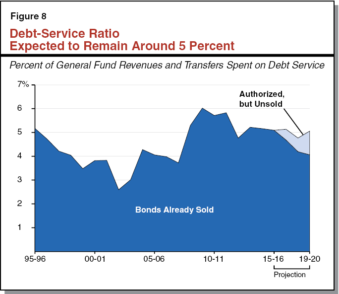
DSR Expected to Remain About 5 Percent. We estimate that the DSR will remain about 5 percent over the next several years. This is because we project that General Fund revenues and debt–service costs will increase at roughly the same rate over the projection period. We assume that the state gradually sells bonds that have been approved by voters or the Legislature. These bonds include some of the remaining unsold infrastructure bonds that voters approved in 2006 and 2008, as well as a portion of the water bond approved in November 2014 (Proposition 1). We note that water bond sales are expected to occur over a number of years, so the water bond’s full annual debt–service costs will not occur until after the forecast period. Our projections do not include any additional debt–service costs for new bonds that may be authorized by the voters or the Legislature during the forecast period.
Chapter 4: The General Fund After 2016–17
In this chapter, we present the results of our multiyear budget outlook. First, we describe the future condition of the General Fund budget under our main scenario, which assumes the economy grows through 2019–20. Because the economy will not grow indefinitely, we then present alternative scenarios sketching the potential effects of an economic slowdown and a recession. We stress that these illustrative scenarios are meant to provide legislators a rough sense of future budget conditions under various economic scenarios. Finally, we describe various non–economic risks that apply to all scenarios. The Appendix at the end of this chapter lists the key results of our multiyear budget outlook, including the alternative scenarios we discuss below.
Key Definition: Operating Surpluses and Deficits. In this chapter, we define operating surpluses or deficits as increases or decreases in the state’s total reserves each fiscal year in its two main reserve funds—the Budget Stabilization Account (BSA) and the Special Fund for Economic Uncertainties (SFEU). The SFEU is the state’s traditional General Fund budget reserve, the funds in which the Legislature may use for any purpose. The BSA is the rainy–day fund created by Proposition 58 (2004) and modified by Proposition 2 (2014).
Main Scenario
Operating Surpluses Assuming Continued Economic Growth. Figure 1 displays operating surpluses under our main scenario. If current laws and policies remain in place, the General Fund would be in surplus through 2019–20. BSA deposits would be available only for future budget emergencies, as defined by Proposition 2. The remaining SFEU surplus would be available for new budget commitments—including spending increases or tax reductions—or building larger reserves. The “remaining operating surplus” bars in Figure 1 suggest the General Fund could afford more than $2 billion in additional annual budget commitments, but only if the economy continues to grow as our main scenario assumes. Figure 2 also summarizes the condition of the General Fund in our main scenario outlook.
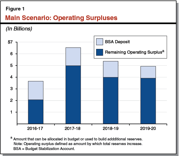
Figure 2
LAO General Fund Condition Under Main Scenarioa
(In Billions)
|
2014–15 |
2015–16 |
2016–17 |
2017–18 |
2018–19 |
2019–20 |
|
|
Prior–year fund balance |
$5.3 |
$2.2 |
$3.2 |
$5.3 |
$10.3 |
$14.3 |
|
Revenues and transfers |
112.2 |
116.3 |
123.2 |
128.8 |
131.3 |
134.5 |
|
Expenditures |
115.3 |
115.3 |
121.1 |
123.8 |
127.3 |
130.6 |
|
Ending fund balance |
$2.2 |
$3.2 |
$5.3 |
$10.3 |
$14.3 |
$18.2 |
|
Encumbrances |
–1.0 |
–1.0 |
–1.0 |
–1.0 |
–1.0 |
–1.0 |
|
SFEU balance |
$1.2 |
$2.2 |
$4.3 |
$9.3 |
$13.3 |
$17.2 |
|
Reserves |
||||||
|
SFEU balance |
$1.2 |
$2.2 |
$4.3 |
$9.3 |
$13.3 |
$17.2 |
|
BSA balance |
1.6 |
5.6 |
7.2 |
8.8 |
10.2 |
11.2 |
|
Total Reserves |
$2.8 |
$7.9 |
$11.5 |
$18.1 |
$23.4 |
$28.4 |
|
aIncludes Education Protection Account created by Proposition 30 (2012). SFEU = Special Fund for Economic Uncertainties (the General Fund’s traditional budget reserve) and BSA = Budget Stabilization Account. |
||||||
Alternate Scenarios
Illustration of Outcomes if Economy Does Not Grow Through 2019–20. As we discussed earlier, our main scenario assumes continued economic growth and modest stock market gains through 2019–20. If this occurred, it would represent the longest expansion in U.S. history. Given that some type of economic or stock market downturn is possible during the outlook period, we assess the budget’s ability to weather economic conditions that are worse than portrayed in our main scenario. Specifically, we consider a hypothetical scenario in which economic growth slows down beginning in 2017 and another hypothetical scenario in which a recession occurs. The nearby box outlines the assumptions in these alternative scenarios.
Key Assumptions in Our Alternative Scenarios
There are four inputs to these scenarios: revenues, Proposition 98, Proposition 2, and other spending. Relative to our main scenario, each alternative assumes lower personal income tax revenues, including lower revenues from capital gains. For the purposes of calculating the Proposition 98 minimum guarantee, we assume local property tax revenues are unchanged but assume slower growth in per capita personal income. These assumptions result in lower Proposition 98 spending. Similarly, lower capital gains taxes reduce Proposition 2 requirements. Lastly, because health and human services caseloads generally increase when the economy worsens, we assume higher net spending in these programs.
Slowdown Scenario
State Still Has Operating Surpluses, Though Much Smaller. Figure 3 displays the result of our economic slowdown scenario. Relative to our main scenario, we assume revenues are almost $30 billion lower over the four fiscal years combined. Specifically, revenues are several billion dollars lower for the first two fiscal years, $10 billion lower than the main scenario in the third fiscal year, and begin to recover in the final fiscal year of the scenario. More than half of the revenue loss is offset by lower spending and reserve requirements under Propositions 98 and 2. In this way, these budget formulas serve as “automatic stabilizers” that mitigate revenue losses. This would, however, also mean that school and community college spending would be notably lower than under our main scenario. While operating surpluses are much smaller than under our main scenario, total reserves remain above $10 billion in each year over the period. The budget is much better prepared to withstand an economic slowdown than it was even one year ago, when we discussed a similar slowdown scenario in this publication.
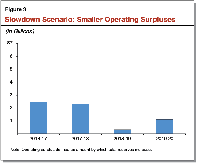
In the slowdown scenario described above, we assume that no new additional commitments are made in the 2016–17 budget. We also considered what would happen in this slowdown if we assume an additional $2 billion in ongoing budget commitments are made beginning in 2016–17. This would eliminate the small operating surpluses in 2018–19 and 2019–20 shown in Figure 3. While the state would have to use its reserves to cover deficits in those years, the total reserve balance would still be over $6 billion at the end of 2019–20. The budget, therefore, appears to be in a position to withstand an economic slowdown even if some additional budget commitments are made next year.
Recession Scenario
We next explored the potential effects of a recession approaching the severity of the dot.com bust of the early 2000s. Under this scenario, a hypothetical recession begins in 2017, and revenues are nearly $60 billion lower over the four fiscal years combined. Specifically, revenues are a few billion dollars lower than in the main scenario in 2016–17, $18 billion lower in 2017–18, $20 billion lower in 2018–19, and $16 billion lower in 2019–20. As shown in Figure 4, deficits return in 2017–18, but reserves are sufficient to cover them until 2019–20. In that year, reserves cover roughly half of the 2019–20 shortfall, with actions necessary to address a $2.4 billion remaining budget problem. The budget fares well in this scenario because we assume no new commitments in 2016–17, allowing the state to build over $9 billion in total reserves before the major revenue losses occur in 2017–18. In addition, lower spending and reserve requirements under Propositions 98 and 2 offset over half of this revenue loss.
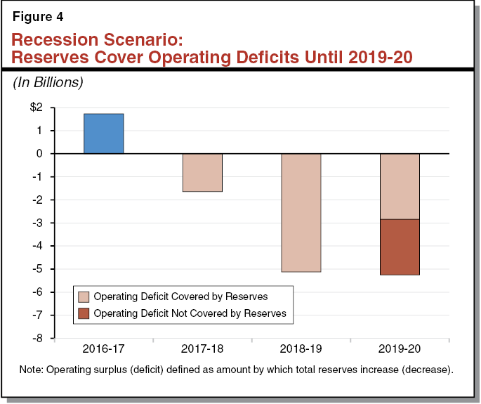
The budget outlook under the recession scenario would be worse if the state makes new ongoing budget commitments in 2016–17. For example, we considered what would happen in the hypothetical recession if $2 billion in new, ongoing budget commitments were made in 2016–17. In that case, the state would face operating deficits one fiscal year earlier than shown in Figure 4. By 2019–20, the state would face a roughly $7 billion budget problem with no reserves.
Risks
Economic uncertainty is only one of many risks to consider in budgetary planning. We detail some of these other risks below.
Pension Costs Could Be Billions Higher. In recent months, the state’s two key pension boards—California Public Employees’ Retirement System (CalPERS) and California State Teachers’ Retirement System (CalSTRS)—have been considering proposals to reduce risk in their investment portfolios. CalPERS has yet to adopt a proposal. CalSTRS, on the other hand, recently adopted a plan to gradually move a small part of their portfolio to less risky investments. If the boards determine that these investment strategies or other factors should be accompanied by lower investment return assumptions, combined state contributions to CalPERS and CalSTRS could be billions of dollars higher by 2019–20 than our estimates. The precise effect would depend on (1) the magnitude of the change in assumptions, and (2) how quickly these changes were implemented. While these changes could hurt the state budget over the next few years, they could lower costs in future decades.
Employee Compensation and Retiree Health Costs Could Be Higher. Next year, the Legislature may be asked to ratify memoranda of understanding with up to 18 bargaining units representing more than 95 percent of the state’s General Fund employee compensation costs. Our main scenario assumes that these employees receive pay increases based on increases in the cost of living. Our estimates do not reflect, however, the Governor’s proposal to prefund retiree health benefits through the bargaining process. This policy could increase General Fund costs by a few hundred million dollars per year above the estimates reflected in this report. (Some or all of these retirement costs could be paid using Proposition 2 debt payment funds.) To the extent that salary increases offset employees’ costs of prefunding, state costs could be even higher.
Assumes Revenue Provisions Not Triggered. California has three budgetary rules—a constitutional spending limit passed in 1979 and two sales tax statutes—that require rebates to taxpayers or tax rate reductions in certain circumstances. None of our scenarios assume rebates or tax reductions occur. Yet, there is a chance that either or both could occur before 2020. The state’s headroom under its complex spending limit has fallen significantly in recent years. Further, larger balances in the SFEU could trigger sales tax reductions. The longer the economic expansion and the larger the reserve balance grows in the SFEU, the greater the chance that tax rebates or reductions will occur before 2020.
Assumes State Prevails in Lawsuits. The state is involved in various lawsuits that pose risks to our multiyear outlook. One case concerns the rules governing how corporations apportion income to California for tax purposes. Another case concerns the state’s use of proceeds related to the 2012 national mortgage settlement. Consistent with our past practice, we generally assume that the state prevails in these and other lawsuits. If the state is unsuccessful in these cases, the potential budgetary exposure could be in the hundreds of millions of dollars in each case.
Conclusion
Consider Trade–Offs When Weighing New Budget Commitments. As history cautions, the current economic expansion will not last forever. If making it through the next economic downturn with minimal disruption to public programs is a priority, a sizable reserve is the key. Less additional ongoing spending on public programs now probably would mean fewer difficult choices about those programs later. While our main scenario indicates that the Legislature would have the capacity for some new one–time or ongoing commitments in the 2016–17 budget, we advise the Legislature to weigh the merits of those new commitments against the potential for larger budget shortfalls when the next economic downturn occurs.
Appendix
Comparing LAO Budget Outlook Scenarios
General Fund and Education Protection Account Combined (In Millions)
|
2015–16 |
2016–17 |
2017–18 |
2018–19 |
2019–20 |
|
|
Revenues |
|||||
|
Total Revenues and Transfers (Before BSA Deposit) |
|||||
|
Main |
$120,350 |
$124,776 |
$130,339 |
$132,704 |
$135,506 |
|
Slowdown |
120,350 |
122,276 |
121,339 |
122,704 |
128,006 |
|
Recession |
120,350 |
120,776 |
112,339 |
112,704 |
119,506 |
|
Spending |
|||||
|
General Fund Spending |
|||||
|
Main |
$115,262 |
$121,119 |
$123,804 |
$127,345 |
$130,575 |
|
Slowdown |
115,262 |
119,815 |
119,045 |
122,385 |
126,882 |
|
Recession |
115,262 |
119,043 |
113,981 |
117,831 |
124,755 |
|
Proposition 98 Minimum Guarantee (General Fund and Local Property Taxes) |
|||||
|
Main |
$69,148 |
$71,447 |
$74,599 |
$75,825 |
$77,468 |
|
Slowdown |
69,148 |
70,215 |
70,180 |
70,937 |
73,382 |
|
Recession |
69,148 |
69,475 |
64,884 |
66,083 |
70,969 |
|
Proposition 98 General Fund |
|||||
|
Main |
$49,444 |
$50,213 |
$52,110 |
$52,376 |
$52,992 |
|
Slowdown |
49,444 |
48,981 |
47,691 |
47,487 |
48,905 |
|
Recession |
49,444 |
48,242 |
42,395 |
42,634 |
46,492 |
|
Total Reserves |
|||||
|
Main |
$7,880 |
$11,537 |
$18,072 |
$23,432 |
$28,363 |
|
Slowdowna |
7,880 |
10,341 |
12,635 |
12,955 |
14,078 |
|
Recessiona |
7,880 |
9,613 |
7,971 |
2,844 |
–2,405 |
|
aThese scenarios implicity assume Proposition 2 budget emergency suspensions or withdrawals in some fiscal years. BSA = Budget Stabilization Account. |
|||||