Volatility of California’s Personal Income
Tax Structure

---

 

Introduction

In this report, we discuss the volatility of California’s personal income tax (PIT) structure. The PIT is state government’s most important revenue source, contributing over two thirds of the state General Fund, which supports schools, universities, major health and social services programs, prisons, and other state‑funded programs. In a February 2017 report, we focused on the volatility of the PIT base—the types of income that are taxable in the state. This report focuses on California’s PIT structure: how its tax rates, deductions, and credits further affect the volatility of its revenue stream.

Specifically, this report discusses:

• California’s PIT structure, including tax rates that apply to different levels of income and important deductions and credits.
• The approximate contribution of different provisions (tax rates, deductions, credits) to the volatility of PIT revenue.
• Some brief perspectives on the implications of PIT volatility.

How Rates, Deductions, and Credits Affect Tax Liabilities

Figure 1 shows how a filer’s state PIT liability is calculated. The process starts by calculating adjusted gross income (AGI) for federal tax purposes. AGI is used as a starting point on the state PIT form. Filers then apply adjustments, deductions, tax rates, and credits to arrive at their tax liability. In this report, we are focused on how these latter steps affect PIT volatility. We detail this process below.

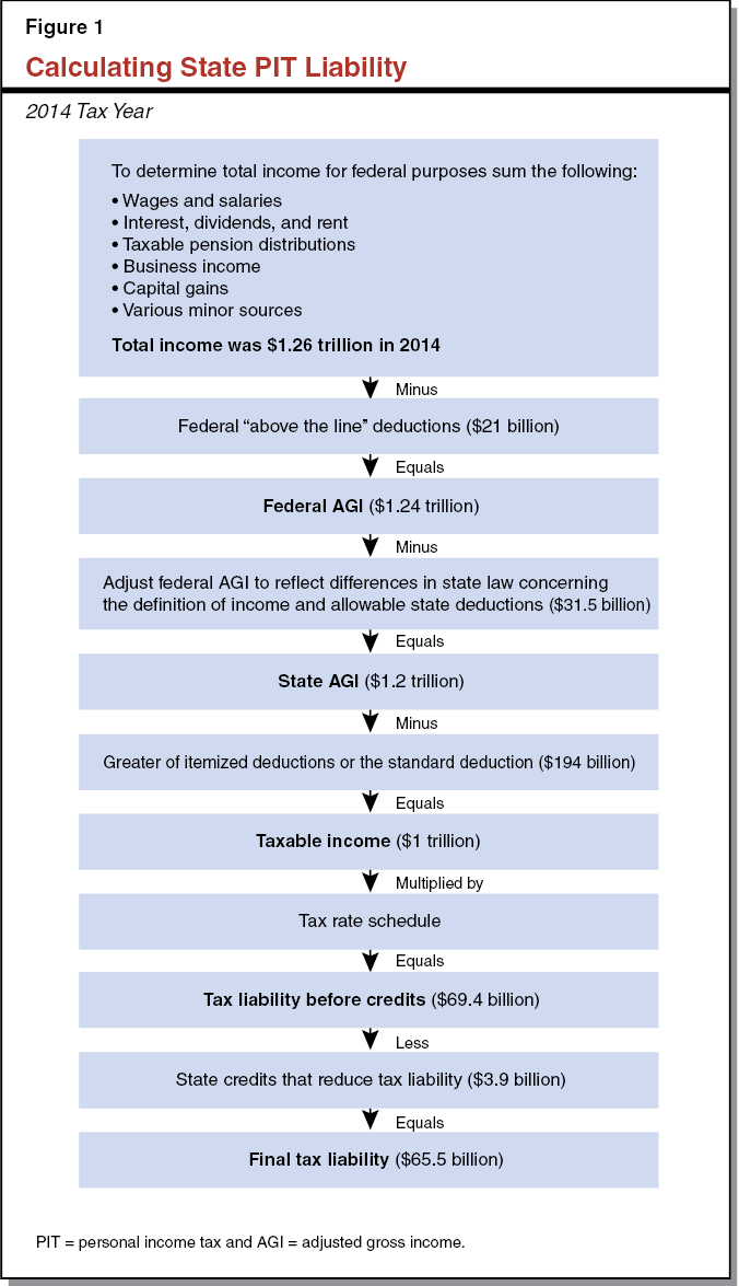
Determining Federal AGI. Calculating federal AGI begins with summing the types of income that are subject to the federal income tax. (A detailed account of the types of income that are in the PIT base can be found in our previous report.) Total income is then reduced by “above the line” deductions. The federal income tax code has a number of deductions that taxpayers are allowed to claim regardless of whether they claim itemized deductions or the standard deduction. As the name suggests, above the line deductions are calculated above the line on the federal tax form that separates the section where AGI is determined from the section where taxable income and tax liability are determined. (Because filers are not required to report above the line deductions on state returns, there are no state data showing how much was claimed in any year. For this report, we have estimated these amounts for taxpayers in different income brackets based on Internal Revenue Service data for above the line deductions claimed by California taxpayers on their federal returns.)

Determining State AGI. For the most part, the definition of income for tax purposes under California law is the same as under federal law. There are some exceptions, the biggest of which is that Social Security income is partially taxable at the federal level but tax‑free at the state level. As the state income tax return starts with federal AGI, it is often necessary to make some additions and subtractions to arrive at state AGI. On net, these adjustments resulted in state AGI being $31.5 billion lower than federal AGI in 2014. Relative to federal AGI, these adjustments reduce state AGI for lower‑income filers with relatively stable incomes and increase state AGI for taxpayers making more than $400,000.

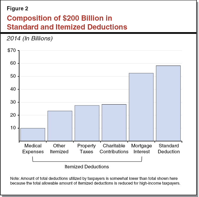
Itemized or Standard Deductions. From state AGI, taxpayers deduct the greater of the total of their itemized deductions or the standard deduction for their filing status (single, married filing jointly, head of household, etc.). A filer who itemizes cannot claim the standard deduction, and likewise a filer who claims the standard deduction gets no benefit from their itemized deductions. Figure 2 shows a breakdown of the $200 billion in standard and itemized deductions claimed in 2014, which reduced taxable income to about $1 trillion.

Marginal Tax Rates. The next step is to apply the marginal tax rates to the filer’s taxable income to determine the filer’s liability before credits. The state PIT uses a graduated rate system, meaning that the rate that applies to each portion of a filer’s income increases as the filer’s income itself increases. As shown in Figure 3, in 2016 the first $8,015 of a single filer’s taxable income is taxed at a 1 percent rate, the next $11,001 is taxed at 2 percent, and so on.

Since voters passed Proposition 30 in 2012, the state has imposed an additional tax of up to 3 percent on high‑income taxpayers (the three highest brackets shown in Figure 3). All revenue from these additional rates is deposited into the state’s General Fund. While these rates are in effect only through 2030, we include their impacts on volatility in this report. (There is an additional 1 percent tax rate on income over $1 million that goes into a special fund to pay for mental health services. As this report focuses on the volatility of the General Fund, this 1 percent rate is excluded from the discussion of tax rates.)

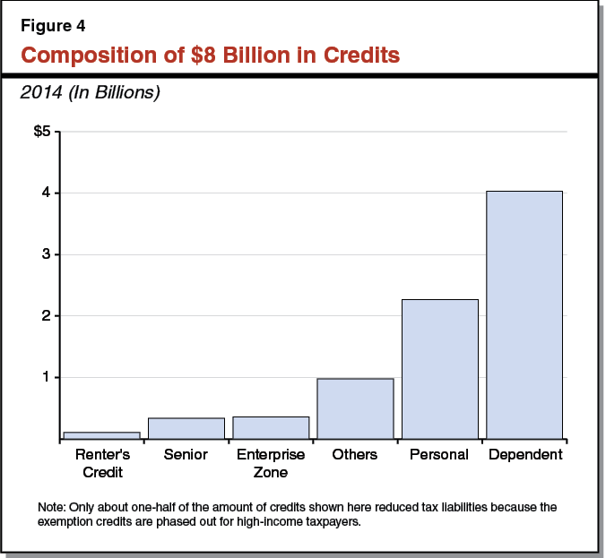
Credits. A credit is a provision that directly reduces a filer’s tax liability instead of reducing their taxable income the way a deduction does. As shown in Figure 4, the two credits that reduce revenue the most are those credits for individuals and dependents. In 2016, these credits were worth $111 for each filer ($222 for a joint return) and $344 for each dependent.

Measuring Volatility

There are many ways to measure volatility. One such measure is average deviation (AD), which was also used in our previous report. AD summarizes how annual observations deviate from the average annual compounded growth rate over a period of years.

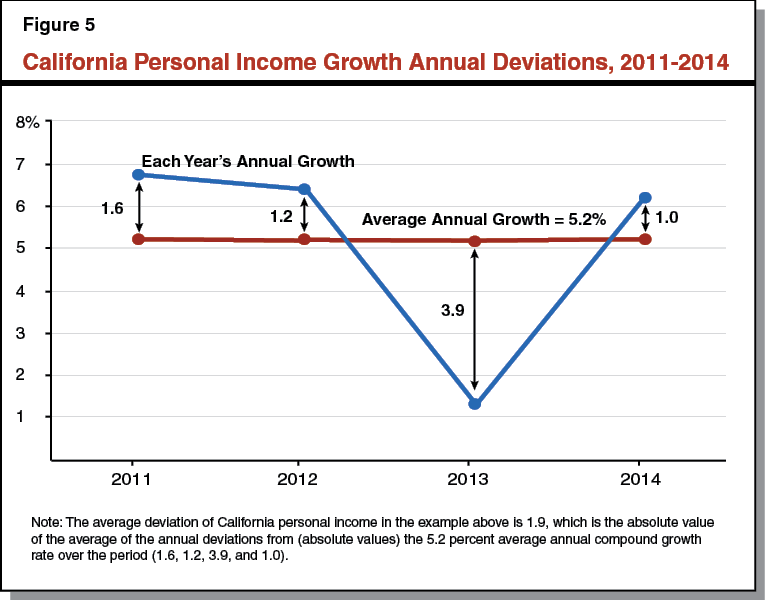
Figure 5 illustrates AD for California’s personal income growth between 2011 and 2014. The compound annual growth rate over this four‑year period was 5.2 percent, as shown by the red line. The growth rate in 2011 was 6.8 percent, which is 1.6 percentage points above the compound annual growth rate, so the annual deviation for 2011 is 1.6. Because the sum of positive and negative deviations is usually approximately zero, the AD calculation has to use the absolute value (always a positive number) of each annual deviation. For example, in 2013 the growth rate was 1.3 percent, or 3.9 points below the 5.2 percent average annual growth rate, but the annual deviation is positive 3.9. The average of all four annual deviations in Figure 2 (1.6, 1.2, 3.9, and 1.0) is 1.9 percentage points, which produces an AD of 1.9. This means that if the pattern that held from 2011 to 2014 continues into the future, personal income growth would deviate from its average growth rate by an average of (plus or minus) 1.9 percentage points each year. The higher the AD of an income or tax, the more volatile it is—tending to move more up or down each year, compared to the average annual growth rate over time.

AD of PIT Tax Structure

Comparing Personal Income Volatility to PIT Volatility. In our previous report, we calculated the AD of personal income to be 2.3. To determine the causes of PIT volatility, we first estimate the AD of the overall PIT and compare it to the AD of personal income. We calculate that the state’s current PIT has an AD of 12.2. (To control for tax law changes, we estimated how much General Fund revenue would have been collected in each year from 1990 to 2014 if the 2016 tax structure had been in place over the entire period.) In other words, revenue from the PIT is more than five times as volatile as personal income itself. Below, we discuss the sources of the 9.9 AD difference between the 12.2 AD of the current PIT and the 2.3 AD of personal income.

Volatility From the PIT Base. In our previous report on PIT volatility (Volatility of the Personal Income Tax Base), we found that the current PIT tax base has an AD of 6.3. This means that the base is almost three times as volatile as personal income. The 4.0 difference in AD explains about 40 percent of the 9.9 AD difference between personal income and PIT.

Volatility From the Graduated Rate Structure. To estimate the volatility of the rate structure, we calculate the AD of a hypothetical PIT with a single rate. We estimate that a single tax rate of 6.23 percent with all deductions, adjustments, and credits kept the same as under current state law would have raised as much revenue from 1990 to 2014 as the actual 2016 tax structure would have. The estimated AD of the state PIT under this flat‑rate scenario was 8.2, or 4.0 points less than the AD of the 2016 PIT structure. From this we can conclude that imposing a graduated rate structure instead of a flat rate adds about 4 points to the AD of the tax.

Volatility From Deductions and Credits. We estimated a hypothetical PIT, with a graduated rate structure proportional to the 2016 rates, but with no deductions, adjustments, or credits, that would have raised as much revenue from 1990 to 2014 as the current PIT structure. This resulted in a rate of 0.685 percent on the current 1 percent bracket, a rate of 1.37 percent on the 2 percent bracket, and so on. The estimated AD of the state PIT under this scenario was 10.1, or 2.1 points below the AD of the current PIT structure. We estimate that roughly three‑quarters of this 2.1 point gap comes from deductions, and the remainder from credits.

Understanding the Volatility of the PIT Structure

Below, we explain why rates, deductions, and credits increase PIT volatility.

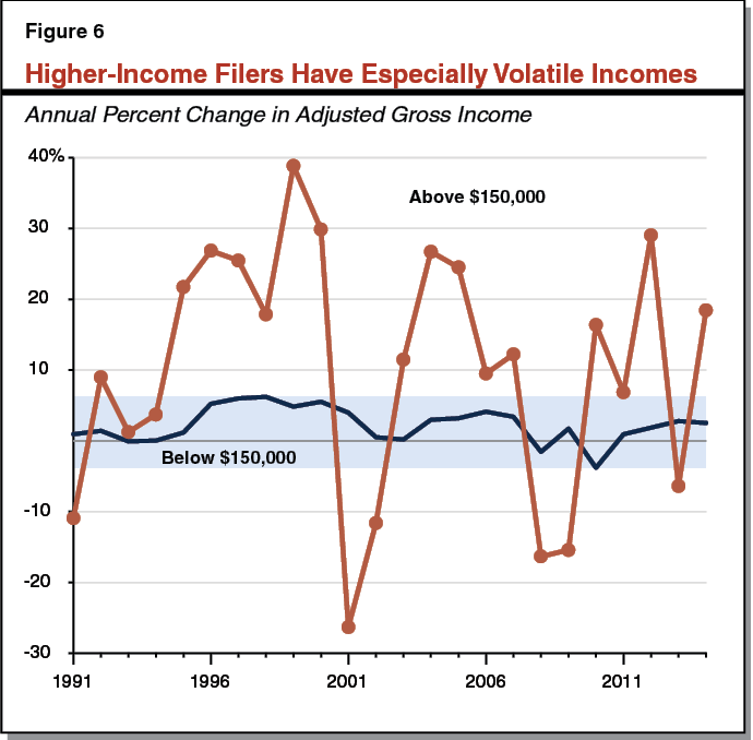
Income Dynamics Differ Above, Below $150,000 a Year. The year‑to‑year volatility in people’s incomes depends where they are on the income spectrum. For instance, for those earning above $150,000 (roughly the top 10 percent of filers in 2014), their aggregate incomes over the past 25 years had an AD of 14.2. By comparison, aggregate income below $150,000 a year had an AD of 2.0. This means that the aggregate income of higher‑income filers is more than seven times as volatile as income of lower‑income filers. As Figure 6 shows, aggregate income below $150,000 is remarkably stable—the period from 1990 to 2014 included some very strong economic years and some very weak ones, yet the growth rate of income below $150,000 was never higher than 6.2 percent or lower than minus 3.8 percent.

How Do Graduated Rates Promote Volatility? As Figure 3 earlier showed, much of the first $150,000 of a filer’s income is taxed at rates below 9.3 percent. In fact, in 2014 over 80 percent of filers below $150,000 would have had no income taxed at the 9.3 percent rate even if the state’s tax code had no deductions or credits. In contrast, most of the income of filers above $150,000 is taxed at rates ranging from 9.3 percent to 12.3 percent. As aggregate income of filers above $150,000 is highly volatile, the graduated rate structure causes PIT revenue to be more volatile than it would be under a single rate. In other words, the rate structure amplifies the impact of the already volatile income of higher‑income taxpayers.

How Do Deductions Increase Volatility? In theory, deductions can affect PIT volatility in different ways, depending on how much they vary from year to year and whether they tend to move in the same direction as AGI. In practice, however, aggregate deductions increase volatility because they disproportionately benefit lower‑ and middle‑income filers as opposed to higher‑income filers and because they are less volatile than AGI. (If deductions were more volatile than AGI, they could reduce overall volatility by reducing taxable income much more in years when AGI is high than in years when it is low.) Filers with incomes under $150,000 claimed 79 percent of total deductions in 2014. This reduces the stable portion of the PIT base much more than the volatile portion, and makes the remaining PIT structure relatively more volatile. Of the six largest deductions, only the deduction for charitable contributions primarily benefits upper‑income people. In contrast, filers below $150,000 a year claimed 75 percent of deductions for mortgage interest (the largest itemized deduction), 93 percent for medical expenses, and 98 percent of standard deductions.

How Do Credits Increase Volatility? By shrinking the stable portion of the PIT base more than the volatile portion, aggregate deductions increase the volatility of the overall PIT. Similar to deductions, credits increase volatility because they primarily benefit lower‑ and middle‑income filers and because they are less volatile than AGI. In 2014, 75 percent of total credits—including 89 percent of personal, dependent, senior, and blind ‘exemption’ credits—went to filers below $150,000 in income. The state’s other credits that are mostly available to filers with business income went primarily to upper‑income filers, but these accounted for a small percentage of the total. Similar to deductions, credits disproportionately reduce incomes of lower‑income taxpayers, thereby increasing overall volatility of the system by making it more reliant on higher‑income tax payers.

Conclusion

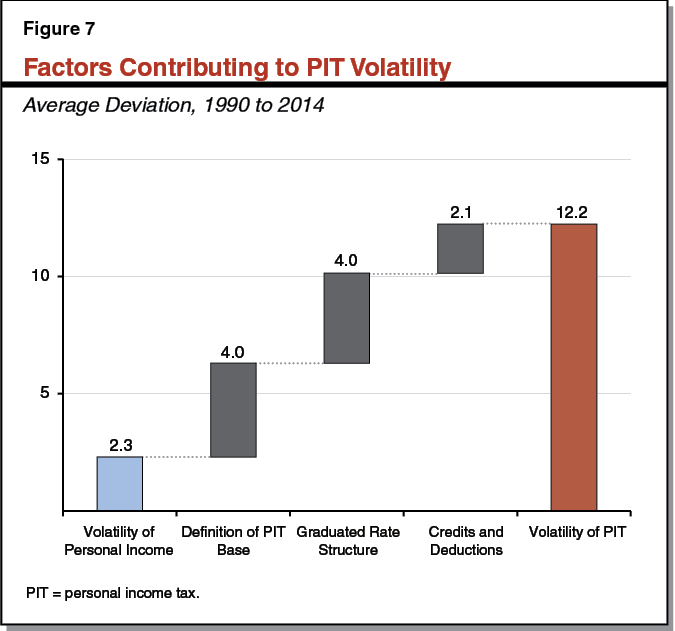
Summary of PIT Volatility. Figure 7 shows the factors that make the PIT more volatile than personal income. As mentioned above, personal income has an AD of 2.3 compared to 12.2 for the PIT itself. Roughly 40 percent of this additional volatility comes from the differences between personal income and the PIT base, another 40 percent from the state’s progressive rate structure, and the final 20 percent from the state’s system of deductions and credits.

State PIT Base Much More Volatile Than Personal Income. Why is the PIT base so much more volatile than personal income? About half of the difference comes from capital gains being included in the PIT base but excluded from personal income. Capital gains have an AD of 35.3—nearly three times the volatility of today’s overall PIT. The other half of the difference arises because some relatively stable income categories—including employer‑paid benefits, transfer payments like Social Security and unemployment insurance, and the excluded components of dividends, interest, and rent—are excluded from PIT. Moreover, transfer payments tend to rise during recessions when other categories of income decline, so they serve to smooth out aggregate income from one year to the next.

Why Do Graduated Rates and Other Provisions Make the PIT More Volatile? California’s graduated rate structure that taxes higher‑income filers more heavily than lower‑income filers makes PIT revenue more volatile. This is the case because aggregate income reported by high‑income filers has been much more volatile than aggregate income reported by low‑income filers. By taxing higher‑income filers at higher rates, the graduated rate structure amplifies the volatility of taxes paid by these filers. This pattern seems likely to continue barring a fundamental shift in the economy. Upper‑income filers get a disproportionate amount of their income from business profits and capital gains, which are especially volatile. Deductions and credits also increase estimated volatility. This is mainly because they mostly benefit lower‑ and middle‑income filers, and thereby reduce the relatively stable part of the PIT base proportionately more than they reduce the relatively volatile piece of the PIT base.

Legislature Could Reduce PIT Volatility . . . The state’s choices about what to include in (and exclude from) its tax base make the PIT tax base more volatile than state personal income. Likewise, the state’s adoption of a steeply progressive PIT rate structure and various deductions and credits cause PIT revenue to be about twice as volatile as the tax base itself. The Legislature has control over most aspects of the base and structure of the PIT and could take any number of steps to reduce its volatility (in addition to the recent adoption of Proposition 2, which, as discussed in our prior report, aims to manage state budget volatility). In evaluating any proposed change, policymakers should also consider potential impacts on taxpayer behavior, on the incidence of the tax, and on ease of compliance and administration (especially if the state deviates from federal policy).

. . . But More Stable PIT Would Likely Come at Cost of Less Revenue Growth. We have discussed how the state PIT’s progressive rate structure increases volatility because the aggregate income of high‑income people is especially volatile. It has also been the case that on average, the aggregate income of high‑income people has grown much faster than the income of the whole population. If the PIT had been less reliant on high‑income filers, it would have been less volatile but it also would have grown more slowly.