November 2007

Tax Expenditure Reviews

(Prepared for the Senate Committee on Revenue and Taxation Assembly Committee on Revenue and Taxation Joint Legislative Budget Committee.)

Introduction

The Supplemental Report of the 2006–07 Budget Act requires the Legislative Analyst’s Office (LAO) to report to the chairs of the Senate Committee on Revenue and Taxation, the Assembly Committee on Revenue and Taxation, and the Joint Legislative Budget Committee regarding tax expenditure programs (TEPs), as specified. Such TEPs are features of the tax code—including credits, deductions, exclusions, and exemptions—that enable a targeted set of taxpayers to reduce their taxes relative to what they would pay under what policymakers perceive to be a “basic” or “normal” tax–law structure. Individual TEPs have been adopted for a variety of reasons, but most exist in order to encourage certain types of behavior by individuals and/or businesses or to provide financial assistance to certain taxpayers.

The supplemental report language requires us both to provide information on newly enacted TEPs and to review selected existing TEPs for their effectiveness and efficiency. In response to these requirements, we provide the following:

• Summary information on recently enacted TEPs.
• More extensive reviews of the two most significant newly enacted TEPs (related to housing tax credits and ultra–low sulfur fuel).
• A review of a Sales and Use Tax (SUT) TEP related to bunker fuel (as required by a separate statutory provision).
An in–depth review of one of the state’s largest TEPs—the mortgage interest deduction under the personal income tax.

Newly Enacted TEPs

Figure 1 summarizes information on TEP–related law changes that have occurred over the last five years. As the figure shows, we have divided these changes into two categories—minor and major provisions—which we discuss further below.

Minor TEP–Related Provisions

Many existing TEPs have been modified to some degree in recent years. These modifications cover a wide range, including definitional changes, changes in the amount of TEP–related benefits provided by a program, and administrative changes in how a program is managed or operated.

Definitional Changes. Recent definitional changes have allowed new groups of taxpayers to be covered under several existing TEPs. For instance, several recent bills have added new events to the list of those qualified for receiving disaster loss tax treatment. Similarly, definitions of excludable victim compensation have recently been expanded to include a broader class of payments to Holocaust survivors as well as payments related to Armenian genocide. Another recent change added certain mutual water company mergers to the list of transactions qualifying as tax–free reorganizations. These and other definitional changes are not new TEPs, however, since they only add participants but do not fundamentally modify the TEPs’ underlying nature.

Figure 1 Recent TEP-Related Law Changes
Statute			Tax	Description
Major
Chapter 786, Statutes of 2004 (AB 2846, Salinas)			PT	Excludes low-income housing tax credits from the income method of property appraisal.
Chapter 691, Statutes of 2005 (AB 115, Klehs)			PIT, CT	Credit for small refiners of ultra-low sulfur diesel.
Minor
Definitional Changes
Disaster Losses
Chapter 772, Statutes of 2004 (AB 1510, Kehoe)			PIT, CT, PT	Disaster loss treatment for various disasters.
Chapter 624, Statutes of 2005 (AB 18, LaMalfa)			PIT, CT, PT	Disaster loss treatment for Shasta County wildfires.
Chapter 623, Statutes of 2005 (AB 164, Nava) Chapter 622, 2005 (SB 457, Kehoe)			PIT, CT, PT	Disaster loss treatment for severe rainstorms in nine counties.
Chapter 222, Statutes of 2007 (SB 38, Battin) Chapter 223, Statutes of 2007 (SB 114, Florez) Chapter 224, Statutes of 2007 (AB 62, Nava)			PIT, CT, PT	Disaster loss treatment for freeze of 2007 and various wildfires in 2006 and 2007.
Chapter 225, Statutes of 2007 (AB 297, Maze)			PT	Temporary PT exemption for replanting fruit trees damaged by the freeze of 2007.
Victim Compensation
Chapter 701, Statutes of 2002 (AB 989, Chan)			PIT	Excludes Holocaust restitution payments from income.
Chapter 807, Statutes of 2002 (SB 219, SRT)			PIT	Exempts certain income items related to disasters or acts of terrorism.
Chapter 402, Statutes of 2004 (SB 1689, Poochigian)			PIT	Excludes Armenian genocide restitution payments from income.
Other
Chapter 1108, Statutes of 2002 (SB 1977, Johannessen)			CT	Tax-free reorganizations of certain mutual water companies.
Benefit Changes
Chapter 34, Statutes of 2002 (AB 1122, Corbett) Chapter 35, Statutes of 2002 (SB 657, Scott)			PIT	Increased contribution limits for retirement and education accounts.
Chapter 580, Statutes of 2006 (AB 2831, Ridley-Thomas)			PIT, CT	Increased cap for Community Development Financial Institution Credit.
Administrative Changes
Chapter 718, Statutes of 2005 (AB 1550, Arambula)			PIT, CT	Designation and standardization of benefits in economic development areas.
Chapter 34, Statutes of 2002 (AB 1122, Corbett) Chapter 35, Statutes of 2002 (SB 657, Scott)			PIT	Administration of retirement and education savings accounts.
Chapter 552, Statutes of 2004 (SB 1713, Machado)			PIT	Expansion of favorable tax treatments provided to military personnel.
TEP = tax expenditure program; PT = property tax; PIT = personal income tax; CT = corporation tax; SRT = Senate Revenue and Taxation Committee.

Benefit Changes. Other recent tax–law changes have increased the size of the benefits available for existing TEPs. Such changes involve increasing annual contribution limits for a variety of tax–favored retirement and education accounts. Also, the cap on the aggregate annual amount of deposits qualifying for the Community Development Financial Institution Credit was increased from $10 million to $25 million.

Administrative Changes. Finally, administrative changes have been made to many TEPs. For example, changes were made last year to the methods for designating and defining various types of economic development areas, as well as standardizing some of the tax benefits available within different types of these targeted geographic areas. Again, these changes did not affect the fundamental nature or approach of these TEPs, which continue to use the same basic tools to promote local economic development. Other TEPs whose administration has been affected by recent legislation include: retirement savings accounts, education savings accounts, and certain favorable tax treatments provided to military personnel.

Tax Changes Constituting Major New TEPs

Two programs created since 2002 constitute significant new TEPs. They are: (1) a modification of the income method of property appraisal so as to exclude low–income housing credits and (2) an ultra–low–sulfur diesel refining income tax credit. We discuss these TEPs in greater detail in the following two sections.

The Ultra–Low–Sulfur Diesel Fuel Credit

Background

Regulations Regarding Low–Sulfur Diesel Fuel

Federal and state regulations that took effect July 1, 2006, require refiners that produce diesel fuel for use in highway vehicles in the United States to achieve a sulfur content not in excess of 15 parts per million by weight. California regulations also extend this limitation on maximum sulfur content to diesel fuel produced for off–highway use. These sulfur content regulations were imposed to reduce the environmental damage caused by sulfur emissions.

Federal Tax Subsidies for Low–Sulfur Diesel Fuel

As part of the American Jobs Creation Act of 2004, the federal government created various tax provisions to ameliorate the cost of retrofitting existing refineries to produce the new, lower–sulfur diesel fuel mandated by federal regulations. These provisions included both accelerated depreciation for certain refining investments and a tax credit for qualified fuel production.

The New State Tax Credit Program

Chapter 691, Statutes of 2005 (AB 115, Klehs), created a new state tax credit for the production of ultra–low–sulfur diesel fuel under both the personal income tax (PIT) and corporation tax (CT). It provides partial state compensation for costs incurred by qualifying refiners as a result of government regulations. Its key provisions are as follows:

• The credit is equal to 5 cents for each gallon of diesel fuel produced, but is limited to 25 percent of qualified capital costs incurred for environmental compliance.
• Qualified investments must have been made in response to federal Environmental Protection Agency or California Air Resources Board (CARB) regulations, and must have been made between January 1, 2004 and May 31, 2007.
• Unused credits may be carried forward for use in future income years if and when taxpayers have sufficient income to use them, but the carryforward provision sunsets December 31, 2017.
• The credit is limited to small refiners, defined as those that process less than 55,000 barrels of crude oil per day.
There is a recapture provision under which taxpayers must repay a portion of the credits they have received if a refinery is sold within five years of having qualified for the credit.

Chapter 691 also conformed state law to federal provisions for accelerated depreciation of qualified refining investments. As discussed earlier in the introductory portion of this report, we classify these depreciation provisions as an expansion of existing rules on accelerated depreciation rather than as a new TEP.

Rationale for the TEP

Economists generally argue that, barring special considerations, producers of goods and services—and not the government or taxpayers at large—should ordinarily be responsible for the costs incurred in providing them. This includes any adverse by–products (which economists commonly refer to as “negative externalities”) of their production activities, such as causing environmental damages. This would argue against providing a state credit to producers of low–sulfur diesel fuel to offset their costs of investments needed to comply with government environmental regulations. The fact that most diesel fuel producers do not get such state credits is consistent with this view.

The issue regarding this credit, then, is whether special considerations exist for small refiners to be singled out to have their costs of environmental compliance subsidized by the state’s taxpayers. The main argument for this TEP is that the costs associated with the mandate appear to be disproportionately large for small refiners, largely due to the substantial fixed costs involved in making the required equipment investments. This, in turn, can put small refiners at a competitive disadvantage relative to larger refiners, compared to where they stood before the regulations were imposed.

The relatively large burden that environmental regulations place on small refiners can be seen from basic production and investment data associated with low–sulfur diesel fuel. This includes how the regulations have affected per–gallon production costs and the volumes of mandated investment expenditures that have occurred. For example:

• According to a 2003 CARB report, small refiners account for less than 5 percent of all diesel fuel produced in California.
• In contrast, the small refiners’ share of total costs incurred for installing the newly required equipment was estimated to be between 16 percent and 23 percent—that is, about $40 million of the total costs of between $170 million and $250 million.
Thus, compliance costs per gallon of production are much greater for small refiners. This is true even after reducing the costs to small refiners by 50 percent to account for the combined federal and state tax credits they receive (25 percent each).

What About Operating Costs? Although the TEP does not provide any relief for any increased operating costs associated with mandated investments, it should be noted that these do exist and they, too, are relatively higher for small refiners. The CARB report estimates that the diesel refining industry will bear new ongoing costs due to the regulations, such as for maintaining the new equipment and from increased spoilage of the new product during its distribution. It identifies these costs as being approximately $10 million annually for small refiners and about $60 million annually for the industry as a whole. Thus the ongoing per–gallon cost of the new regulations is also higher for small refiners.

Countering these rationales for the program, there are those who would argue that to the extent small refiners are not efficient producers of ultra–low sulfur fuel when the costs of environmental mitigation are factored in, subsidizing them with a credit means that the government is promoting inefficiency.

Cost of the TEP

Approximately $3 million of this credit was claimed in the 2006 tax year. Due to ownership changes in the refining industry, however, it appears that no new credits will be claimed in future years. In fact, some of the credits already paid out will likely be recaptured, as provided for under the provisions of the program. Thus, the TEP’s ultimate costs will probably be fairly small.

Program Performance and Effects

Little Program Usage Has Occurred

The CARB has identified only one small refiner that qualified for this credit. Furthermore, this refinery was sold approximately two months after receiving certification that its investments qualified for the credit. Under the recapture provisions noted above, this sale means that the refinery no longer qualifies for this credit. The economic activity associated with this refinery’s operations are thus essentially now the same as without the program, and the program’s impacts appear to have been minimal.

Effect on Employment and Production Likely Minimal

A perspective on the program’s effects can be gained by comparing the one qualifying refinery firm’s economic value to the magnitude of the credits it was awarded. According to public records, the refinery that received the $3 million in credits referred to above was sold for $314 million in cash plus $150 million in debt assumption, for a total value of $464 million. If a firm with a market value of $464 million earned, for example, an annual after–tax rate of return of 15 percent, this would translate into annual earnings of roughly $70 million. The $3 million credit earned would increase this return to 15.6 percent, a relatively modest amount, and unlikely to have had a significant effect on firm performance, especially given that the credit is one–time.

Conclusion

Whether a program such as this is desirable depends primarily on how the costs of providing the subsidy compare to the benefits policymakers associate with assisting small refiners with the mandate. These benefits might include maintaining the state’s refining capacity, ensuring that there is a mix of different–sized suppliers active in the industry, and wanting to avoid the short–term economic dislocations of having small refineries possibly go out of business or cut back on their operations as a result of the new requirement.

In considering any state contribution to the costs small refineries face for environmental mitigation, the state should take into account the fact that the federal government is also defraying a portion of these costs. This is being done through both the allowance of accelerated depreciation and the provision of the federal credit. Given this, the state should only provide additional assistance through a state credit if the current federal tax programs do not themselves provide sufficient compensation to the small refiners affected by the new environmental regulations.

In the case of this program, the issue is somewhat academic, in that little use has been made of the credit, what use has occurred has been terminated due to a firm’s sale, and some of the credits previously awarded may be recaptured. Should one or more similar or analogous programs along these same lines be considered at some point in the future, however, the above points may be helpful in crafting them.

Conformity for Its Own Sake Does Not Justify New Credits

One of the principles that this program calls attention to is the circumstances when it may or may not make sense to adopt a TEP for the purpose of conforming state tax law to federal tax law. This particular TEP was one of many provisions included in Chapter 691, which was presented as a conformity bill. There are many situations in which conformity of state and federal tax law is desirable because it can reduce tax compliance costs for taxpayers and administrative costs for state tax agencies. For example, in this same bill, small refiners were also authorized to take accelerated depreciation for their mandated investments, as is provided for by federal law. If the state did not conform to these federal depreciation calculations, taxpayers would incur a substantial burden in calculating depreciation schedules separately for federal and state tax purposes. Thus, an argument for the state adopting accelerated depreciation for small refineries can be made on conformity grounds alone.

This same conformity reasoning does not apply, however, to the adoption of a state credit for low–sulfur diesel fuel. This is because there would be no increase in compliance costs due to federal–state law differences if the state had chosen not to offer this credit. Thus, in cases like this, credits should only be adopted if the TEP would be desirable to California policymakers on its own grounds, not merely in order to conform to federal law.

The Exclusion of Low–Income Housing Credits From the Income Method of Property Appraisal

Background

Low–Income Housing Is Often Appraised Using the Income Method

Property taxes are levied on the assessed value of properties. Assessed values are initially determined by the cost of acquiring a property, with increases of up to 2 percent annually thereafter until the property is resold. According to the California State Board of Equalization (BOE), however, a different method known as the “income method” of appraisal is preferred for assessing low–income housing units. Standard appraisal methods are often not used for low–income housing because these projects are subject to restrictions on their use and resale. These restrictions, in turn, result in lower resale values than would otherwise be expected for comparable properties. Rather than basing property taxes for low–income housing on unattainable values of surrounding property, appraisals using the income method are based on the expected value of the future stream of rental payments from the housing project involved.

Low–Income Housing Credits

The purpose of low–income housing programs is to increase affordability by enabling qualified renters to pay below–market rents for their housing. In order to encourage suppliers to produce and supply low–income housing under these conditions, the government must subsidize suppliers by at least the difference between the rent allowed for these units and the market rent that the suppliers would otherwise have received. One way in which this subsidy is delivered is through low–income housing tax credits.

Both Federal and State Credits Exist. There is a federal low–income housing credit for a percentage of a project’s qualified development costs. There is also a supplemental California state credit. The supplemental state credit is available only to certain projects that are already eligible for the federal credit.

Credit Amounts. Current law provides for two federal low–income housing credits. The first credit, known as the “9 percent credit,” is available only to projects that are not also receiving tax–exempt bond financing. The second credit, the “4 percent credit,” is available to projects that are receiving tax–exempt bond financing. (The exact credit amounts are adjusted periodically and may differ somewhat from 9 percent and 4 percent.) The federal credits are increased by 30 percent for projects in certain locations (known as “Qualified Census Tracts” or “Difficult to Develop Areas”). The supplemental state credit is used to augment the amount of credits available for projects located in areas that do not qualify for the 30 percent federal credit bonus.

Credit Caps. The amount of credits that may be allocated annually for the 9 percent federal credit is capped. California’s 2006 federal limit is about $70 million per year over the following ten years, or approximately $700 million total. The annual allocation of state credits for supplementing the 9 percent credit also is capped—at approximately $70 million total, to be used over the following four years.

The California Tax Credit Allocation Commission in the State Treasurer’s Office is responsible for allocating the available federal and state credit amounts among applicants, based on specified criteria. According to the commission, the demand for the 9 percent federal credit is roughly twice the available amounts.

The amount of the 4 percent credit is not capped directly, but is limited by caps on the underlying tax–exempt financing bonds used by the projects. In 2006, $86 million per year (for ten years) in federal 4 percent credits were allocated to California projects, and $14 million in state credits (allocated over four years) were awarded to supplement these 4 percent credits.

The actual reduction in state revenues in any year due to the program will differ from the amount of credits that have been allocated. This is due, in part, to the use of credits being spread over a four–year period, and, in part, to the fact that the credit is nonrefundable. The latter means that taxpayers who have no tax liability in a particular year must wait to use their credits in a future year for which they do have a tax liability that the credits can offset.

How Credits Should in Theory Affect Appraisals

From an economic standpoint, application of the income method of appraisal would take into account all sources of income that a property receives. As noted above, this would include the expected value of the future stream of rental payments from the housing project involved. It would also include any government subsidy payments that property owners benefit from, whether directly or indirectly. This is because these, too, would be incorporated either fully or partially by the economic marketplace into their properties’ values. This would ordinarily include low–income housing credits. Thus, from a pure tax–policy perspective, such credits would be included in the income method of appraising low–income properties.

The New Tax Exclusion

Chapter 786, Statutes of 2004 (AB 2846, Salinas), created a property tax exclusion under which low–income housing tax credits (both federal and state) are not considered as income to housing suppliers for the purpose of appraising the value of low–income housing property under the income method.

Program Rationale

There are two main rationales offered for this tax provision.

Administrative Uniformity. A primary motivation for this TEP was to improve uniformity in the administration of property taxes. Under law prior to Chapter 786, other government subsidies for low–income housing were explicitly excluded from the income method of appraisal, but tax credits were not. Furthermore, as a matter of practice, while some assessors did include tax credits in their calculations, others did not. Those that did not may have omitted the credits either because they believed that credits were not includable or because they did not have any method for readily identifying those credits that should have been included. The introduction of this TEP provides consistent treatment for developers of low–income housing regardless of the type of government subsidy they receive, and standardizes the actual practice of assessing these properties across counties.

The administrative uniformity rationale for this program raises some issues, however. This is because uniformity in property tax administration with respect to appraisals could be achieved in a different way. For example, uniformity could be reached by having all properties include such credits in the appraisal calculation. In fact, this approach would be more in line with basic tax policy principles. Nevertheless, policy decisions have already been made to exclude noncredit low–income housing subsidies from the income appraisal method. Thus, excluding credits from the income appraisal method is logical if the objective is to treat credit subsidies the same as noncredit subsidies. It is from this perspective, and the fact that all appraisals should be subject to similar rules, that administrative uniformity makes sense as a program rationale for this TEP.

Investment Incentives. The other argument offered by some in support of this program is that it increases the return to investors in qualified low–income housing projects. This could, in turn, maintain and possibly spur additional investments in such projects. As discussed below, this investment incentive is inherently limited in magnitude because of the above–noted caps on the amount of monies budgeted to fund both the federal and state credits.

Cost of the TEP

The BOE estimates that this TEP reduces local property tax revenues by up to $17.5 million annually.

The state budget is also affected by this reduction in local property taxes, in two ways. First, property owners have reduced deductions for property taxes paid when they calculate their PIT or CT. This, in turn, increases state revenues, potentially by up to several million dollars annually. Second, depending on the year in question, the state may be required to increase its contribution toward the minimum K–14 education–funding guarantee under Proposition 98. This is because the state generally backfills, dollar–for–dollar, reductions in the amount of local property tax revenues available to fund the guarantee. Since schools receive over one–third of property taxes statewide, the state cost to backfill the revenue loss from this TEP can be up to $7 million annually.

Evaluation of the TEP

The desirability of the program depends on how its benefits and costs compare—that is, how strongly the Legislature values uniformity in property assessments and the investment incentive for low–income housing relative to the net costs it imposes on the state and its local governments. Valuing the equity benefits of more uniform appraisals is largely a subjective matter that only the Legislature can determine. We discuss further below the potential benefits of the TEP from the investment–incentive perspective.

By excluding the value of low–income housing credits, this TEP reduces the assessed value of the housing units. This has the effect of reducing the annual property taxes paid by owners. (It is important to note, however, that many owners are nonprofit entities that do not pay property taxes and, therefore, this TEP will not benefit them.) How this reduction in annual operating expenses increases the rate of return on such projects would vary depending on their specific characteristics, but it would appear not to have a significant impact.

More importantly, there would appear to be little, if any, production incentive effect from this TEP because of its linkage to the federal and state low–income housing credits. As noted above, these credits are heavily oversubscribed—and were so even before the creation of the income appraisal TEP. As a result, there is a fixed level of investment in these subsidized housing limits each year, and the TEP does not change that level.

Given the above, it is our assessment that the program provides windfall benefits to investors who would already be providing low–income housing without the TEP. Although it is possible that some of this windfall might find its way to housing occupants through lower rents, we think it is far more likely that the windfall accrues entirely to housing suppliers.

Conclusion

In considering the desirability of this program, the Legislature should take into account the following:

• First, how strongly does it value the assessment uniformity the TEP provides? While there are benefits from treating credit and noncredit subsidies equally, uniformity can be achieved either by excluding or including all subsidies in the income method of appraisal.
Second, what are the benefits of the investment incentives the TEP provides for producing more low–income housing? We find these to be insignificant, given the current caps on their availability.

The Legislature should also consider, independent of the above factors, whether additional tax incentives for low–income housing are desired. Depending on the extent that policymakers already selected the appropriate amount of subsidy for low–income housing when the tax credits and other subsidies for low–income housing were put into place, there may or may not be a need to augment these subsidies.

The Partial Sales and Use Tax Exemption for Bunker Fuel

Another TEP adopted in the past five years, but that had existed previously, is the partial SUT exemption for purchases of bunker fuel. The partial exemption was reinstated by Chapter 712, Statutes of 2003 (SB 808, Karnette), which also required the LAO to submit a report assessing the impacts of the partial exemption. The analysis that follows has been prepared in response to this reporting requirement.

Background and Summary

Nature and History of the Exemption

Bunker fuel refers to fuel that is used to propel ships. Like most tangible products sold in the state, bunker fuel is subject to the state’s SUT. However, the state currently provides a partial SUT exemption of bunker fuel sales. Specifically, it does not tax fuel consumed after the first out–of–state destination of the ship has been reached.

California’s tax treatment of bunker fuel has changed back and forth over time. Namely:

• From July 15, 1991 through December 31, 1992, and again from January 1, 2003 through March 31, 2004, the state fully taxed all bunker fuel sales in the state.
On April 1, 2004, pursuant to Chapter 712, California reinstated the partial exemption that had been allowed prior to July 1991 and from January 1, 1993 through December 31, 2002. This partial exemption is now scheduled to sunset January 1, 2014.

Previous LAO Findings on the Exemption

The LAO released a statutorily required study on bunker fuel pursuant to Chapter 615, Statutes of 1997 (AB 366, Havice), entitled Sales Taxation of Bunker Fuel (January 2001). Our major findings were:

• The bunker fuel industry experienced a decline in California in the 1990s.
• The decline stemmed from many factors including: a recession, the temporary revocation of the SUT bunker fuel exemption during this period, declines in refining capacity, changes in shipping technology, and the development of alternative bunker fuel facilities outside of California.
• The revocation of the SUT exemption from July 1991 through December 1992 likely resulted in the loss of 100 to 200 jobs in the industry and increased state–local SUT revenues by a total of between $20 million and $30 million.
A partial exemption for bunker fuel is an appropriate tax policy.

Updated Findings

The fundamentals of the bunker fuel industry and the effects of a partial SUT exemption have not changed since our last report. In our review below, we find that:

• The partial SUT exemption for bunker fuel is still an appropriate tax policy.
• The revocation of the SUT exemption on bunker fuel during 2003 and 2004 produced impacts similar to those that occurred during the early 1990s.
If anything, because of recent increases in fuel prices, revoking the SUT exemption now would likely have an even larger adverse impact than it did previously.

Analysis of the Bunker Fuel Exemption

How Should Bunker Fuel Be Treated From a Tax Policy Perspective?

Underlying Rationale for the SUT. The traditional public finance rationale for the SUT is that the provision of public services by governments facilitates, either directly or indirectly, the conduct of economic activity, including the buying and selling of goods. Thus, this rationale holds, levying a tax on the exchange of goods is a reasonable basis on which to partially fund governmental costs. An important element of this rationale is the presumption that final goods purchased by Californians will also be used in California, and California’s existing SUT provisions generally reflect this philosophy. For example:

• Final purchases by California individuals and businesses for in–state use are taxed unless specifically exempted. Even in instances where the SUT is not collected by sellers or paid by taxpayers—such as on some mail order and Internet sales—this reflects the failure of taxpayers to comply with and remit the tax, not the state’s failure to impose the tax.
Conversely, exemptions are often allowed under the SUT when it is presumed that a good’s regular usage will occur out of state. For example, an exemption is granted for the sale of new or manufactured trucks for out–of–state use.

A Partial Exemption Is Theoretically Sound. Given the above, on tax–policy grounds, a strong argument can be made for the current partial exemption. Generally, items purchased in California that are subject to the SUT are presumed to be used in the state, while sales for export are usually exempt from the SUT. Bunker fuel purchases fall somewhere in between, since bunker fuel purchases are used both outside of and within state boundaries, suggesting that there is a sound basis for a partial SUT bunker fuel exemption.

Fiscal and Economic Effects of the Partial Exemption

The economic and fiscal effects of the bunker fuel SUT exemption—including its impacts on jobs and on state and local tax revenues—depend largely on how it affects the amount and location of bunker fuel sales occurring in California. This, in turn, depends primarily on how the exemption affects bunker fuel prices and the response of shipping companies to price changes. These responses are determined by the relative importance of fuel costs to overall operating costs as well as the flexibility that such shippers have in buying fuel at California versus non–California locations. Understanding these factors requires knowledge about the bunker fuel market’s characteristics and how it functions.

The Bunker Fuel Market—Characteristics and How It Works

The Market Is Relatively Competitive. The bunker fuel market is a global market characterized by a generally standardized product and a high degree of price competition among suppliers. Prices at various ports generally fluctuate in a fairly narrow band although small differences in prices can occur due to supply issues, costs associated with different ports, and other market factors. While some quality differences do exist among different types of bunker fuels, these differences generally are either minimized through the refining or blending process, or more typically, are clearly identified in the contract process and accounted for in the pricing of the fuel.

The market is characterized not only by the fairly significant number of industry competitors, but also from the competitive uses that exist for the residual fuels from which bunker fuel is derived. The residues from the refining process are used to produce various types of fuel oil, only one version of which is bunker fuel. If other types of fuel oil increase in price relative to bunker fuel, bunker fuel production typically declines until the net returns to bunker fuel refinery activities rise and are thereby brought into equilibrium.

In addition, the oil residues can be further distilled, through a more expensive process known as “cracking,” which converts these residues into gasoline or other higher–end products. Again, if price ratios for the different products shift, refineries can adjust their production of the various petrochemical products accordingly. For example, if heavy fuel oils (such as bunker fuel) compare favorably in price to other products, refineries will tend to produce more of these fuels rather than less. Alternatively, given opposite circumstances, refineries will typically crack the residues and “squeeze” more light–end products from the crude oil.

Cost Structure of the Shipping Industry. The shipping industry is highly capital intensive and has substantial fixed costs. (These are costs that are incurred regardless of the exact volume of business undertaken—such as for the ships and related capital equipment.) The industry’s major variable (or operating) costs are labor and fuel. Fuel costs are typically a much larger component of operating costs than are labor costs, representing approximately 60 percent of total operating costs. Thus, at current fuel prices and an average SUT of about 8 percent, a full SUT on bunker fuel would increase total operating costs by about 5 percent.

The combination of multiple bunkering ports and long cruising ranges gives shipping companies considerable flexibility in fueling. Larger loaded ships use on the order of 180 tons to 200 tons per day of bunker fuel. Assuming, as an illustration, that a ship has a fuel capacity of 15,000 tons, this would allow it to cruise for 70 days without refueling, or more than one and one–half round trips across the Pacific Ocean. Ongoing improvements in ship fuel capacity as well as the development of new bunkering facilities would tend to increase the impact that small differences in bunker fuel prices can have on port activities.

Because of the substantial contribution that fuel costs make to the overall expense of ship operations, decisions regarding when and where to bunker are made with close attention to relative fuel prices at different ports. Often, differences of as little as 25 cents to 50 cents per ton can separate losing and winning bids for supplying bunker fuel. The shipping industry has traditionally operated on fairly narrow operating margins, and thus relatively small swings in fuel prices can result in large changes in the financial performance of the shipping industry and its individual companies.

Overall Economic Significance of the Industry. A precise count of the individual jobs and businesses associated with California’s bunker fuel industry is not available. For virtually all of the businesses that participate in the industry, bunker fuel–related activity constitutes only a fraction of their activities. For example, inspectors, tug and barge operators, and fuel dealers are involved in many other markets in addition to the bunker fuel market. Overall, however, it appears as though some two dozen different types of businesses are involved in the industry, with something in the range of 1,000 to 2,000 California jobs being directly linked to the bunker fuel industry.

Recent Historical Experience With Full and Partial SUT Taxation

As noted earlier, from July 15, 1991 through December 31, 1992, and again from January 1, 2003 through March 31, 2004, the state fully taxed all bunker fuel sales in the state. During both of these periods, California bunker fuel sales declined. As reported in our earlier–cited 2001 report, in 1992 bunker fuel deliveries dropped by 45 percent for California ports (compared to declines of about 1 percent for non–California U.S. ports). Likewise, in 2003, bunker fuel sales in Los Angeles and Long Beach (which account for most of California’s sales) dropped 30 percent, and in the first quarter of 2004 they were down 22 percent from a year earlier. In contrast, for the rest of 2004, after the partial exemption was reinstated, sales were up 31 percent over the same three quarters a year earlier, and they increased another 20 percent in 2005. While the partial SUT exemption is only one of many factors influencing total fuel deliveries, both of these experiences suggest that the removal of the partial exemption did result in lost business for California bunker fuel suppliers.

Employment and Revenue Effects. In our earlier report, we estimated possible employment losses of 100 to 200 positions due to the application of the full SUT to bunker fuel sales in the 1990s. Job losses during the 2003–04 period appear to have been similar in magnitude. In addition, revenue increases associated with the state and local SUT are likely to have been in the range of $20 million to $30 million in 1991–93 and $30 million to $40 million in 2003–04. These revenue increases would have been partially offset by declines in other associated fees, such as fuel wharfage and oil spill prevention fees.

Bottom–Line Findings. Based on our review of the performance of the bunker fuel market both with and without the partial exemption in place, we conclude that the partial SUT exemption for bunker fuel increases California bunker fuel sales and related economic activities. At the same time, however, it reduces state and local revenues by tens of millions of dollars annually.

LAO Recommendation

While the Legislature clearly must consider the revenue and economic impacts of any changes in the manner in which it taxes bunker fuel, we believe it is also important for such treatment to be consistent with the conceptual basis of the SUT in general. On tax policy grounds, we believe a strong argument can be made for subjecting such sales only to partial SUT taxation. As discussed earlier, items purchased in California that are subject to the SUT are generally presumed to be used in the state, while sales for export are usually exempt from the SUT. Bunker fuel purchases fall somewhere in between, since bunker fuel purchases are used both outside of and within state boundaries. Consequently, a partial SUT bunker fuel exemption—in our view—approximates the treatment given to most other tangible goods and constitutes appropriate tax treatment.

On this tax policy basis, we recommend that the Legislature remove the existing sunset for the current partial SUT exemption for bunker fuel sales, and make the exemption permanent. This would result in the SUT on fuel purchased in California being levied in the future only on the portion which is consumed between California and a ship’s arrival at its first out–of–state destination (as is currently the case). This action would permanently result in treating bunker fuel sales similarly to other export sales and place California ports on par with other out–of–state ports in the nation.

Mortgage Interest Deduction

In this section, we provide an analysis of the state’s largest TEP—the mortgage interest deduction. We discuss the program’s basic structure and underlying rationale, how its benefits are distributed, and its overall performance. We then offer recommendations for making the program more effective as a policy tool.

Summary and Recommendations

Our principal findings and recommendations are as follows:

• In theory, good tax policy should generally strive to raise revenue without inadvertently causing people to change their behavior. Economists refer to this principle as “economic neutrality.”
• Sometimes, however, tax policies are designed specifically to induce behavioral changes. Such policies may be appropriate when, without intervention, the economic marketplace would produce either too little of a good or service that provides broad social benefits or too much of a good or service that imposes broad social costs.
• Homeownership is one area where many people argue that the free market does not produce an optimal outcome for society as a whole. Their view is that homeowners provide benefits to society by maintaining their homes better and by participating more actively in civic affairs than do renters. According to this view, government policies aimed at increasing the percentage of people who own their own homes may, therefore, be appropriate.
• There are a number of different tax policies that encourage homeownership. The largest is the mortgage interest deduction (MID).
• The MID can be claimed on both federal and California PIT returns. In 2007–08, it is estimated that the state mortgage interest TEP will reduce California tax revenues by approximately $5 billion.
• Under its current structure, the benefits of the MID are poorly targeted. This is because only a small share of its benefits accrues to people who would not own their homes in the absence of this policy, and many of its benefits go to higher–income individuals who purchase expensive homes that arguably should not be subsidized by other taxpayers.
Therefore, we provide several options for improving the effectiveness and efficiency of the MID’s homeownership incentive in the California tax code. We offer both ways to better target the existing deduction and the alternative of replacing the MID with a more limited and better–targeted credit for home purchases.

Organization

In this review, we first briefly discuss the rationale for having the MID. (The Appendix provides background on what the tax code would look like if its primary objective was to provide an economically neutral treatment of housing, and then discusses the case for using the tax code explicitly to encourage homeownership.) Next, we describe current government policies, including several features of the tax code, that affect housing. We then examine the use of one particular provision of the tax code—the MID. We present evidence suggesting that the MID does not effectively and efficiently promote the goal of homeownership. We describe a variety of policy options for more effectively targeting the MID. We then suggest that another alternative—replacing the MID with a credit—would be both more effective and efficient in achieving policy objectives.

Rationale for the MID

California has, for many years, chosen to provide substantial benefits to its homeowners by allowing them to claim a mortgage interest deduction when computing their income taxes. This subsidy to homeowners is similar to the one offered by the federal government and currently costs California taxpayers and the state budget approximately $5 billion annually. Most economists take the view that the tax structure should be “economically neutral” (see discussion in Appendix), meaning that the structure of the tax system should not influence economic decisions unless there are compelling reasons for doing so. In the case of the MID, the primary justification generally offered for providing the subsidy is that homeownership is good for society, and thus should be encouraged.

Current Government Policies Affecting Housing

Housing–Related Tax Provisions

Several provisions of both the federal and California tax codes affect the housing industry. These are discussed below and summarized in Figure 2.

Deductibility of Mortgage Interest. One of the most important provisions of the federal and state tax codes is the MID. Under this provision, taxpayers may claim as an itemized deduction their interest payments on mortgages of up to $1,000,000 for joint filers and $500,000 for single filers on their first and/or second homes, and on home equity loans of up to $100,000 for joint filers and $50,000 for single filers.

Exclusion of Capital Gains on Principal Residences. Another important housing–related tax provision is the exclusion of capital gains on the sale of a principal residence. When taxpayers sell a home that has been their principal residence for two of the previous five years, the first $500,000 of capital gains for joint filers (or $250,000 for single filers) earned on the sale is not included in taxable income.

Basis Step–Up. Although they are not specific to housing, the rules on asset basis step–up at death benefit housing. When an heir sells a house, the capital gains on the sale are calculated from the home’s value at the time of inheritance rather than from its value at the time it was originally purchased.

Deductibility of Property Taxes. The final major housing–related provision of the tax code is that taxpayers may claim an itemized deduction for real property taxes paid on their homes. This deduction is allowed only for property taxes and not for the various other things that can appear on property tax bills, such as specific fees assessed for parks and other public services, landscaping fees, and so–called Mello–Roos fees in California.

Other Provisions. Several other provisions of both federal and California tax law also affect the housing industry, but on a smaller scale than the major programs identified above. For example:

• State housing agencies are allowed to issue tax–exempt bonds and use the proceeds to issue loans at below–market interest rates to low– and moderate–income home buyers.
• The provisions for like–kind exchanges (commonly referred to as Section 1031 exchanges) provide benefits to a variety of taxpayers, including some owners of housing.
An exclusion from income of housing for clergy also exists, and may influence the type of housing occupied by members of the clergy.

Finally, some provisions specific to the California tax code also affect the housing market:

• The California Constitution provides that the assessed value of owner–occupied homes be reduced by $7,000. This results in an annual property tax reduction of approximately $75 per homeowner.
• The California renter’s credit provides a small annual subsidy to lower–income taxpayers.
• The low–income housing credit and the farmworker housing credit subsidize the production of low–income housing.
Lastly, California’s Homeowner’s and Renter’s Assistance Program subsidizes the cost of housing for low–income Californians.

Non–Tax Government Policies Affecting Housing

In addition to the tax–related programs described above, at least two other types of government programs also affect the housing market. First, there are direct expenditure programs aimed at subsidizing low–income housing. This category includes government subsidies for the production of low–income housing (almost all rental units) and government subsidies for rent paid by low–income people. These rent subsidies may encourage a few people to rent rather than own their home, although most of the people receiving these subsidies would probably have been renters anyway due to their income levels.

The government also influences the housing market by regulating the market for mortgages. One important federal influence is through the benefits conferred on government–sponsored enterprises (such as Fannie Mae and Freddie Mac) that help finance mortgages. Also, a number of federal and state agencies insure mortgage loans for particular groups of borrowers. In addition, the state offers mortgage subsidies for qualified first–time homebuyers. These types of government assistance almost certainly encourage homeownership.

Issues to Consider in Evaluating Housing Tax Policy

As described above, both the federal and California governments have adopted a number of policies that influence the housing market. Many (although not all) of these policies are tax expenditures that reduce the taxable income of homeowners and likely, therefore, work to encourage increased homeownership.

The main avenue by which these tax policies work is their overall effect on reducing the cost of acquiring and living in homes, and this reduction appears to be substantial. According to the Final Report of the President’s Advisory Panel on Tax Reform issued in 2006, for example, the tax rate on investment in owner–occupied housing is 14 percent lower than investments generally and this difference flows through to lowering the cost of acquiring housing.

The precise effect of this subsidy on homeownership rates, however, is not clear. A portion of the subsidy may induce some people who would otherwise choose to rent housing to purchase homes. Much of the subsidy, however, likely results in people who would own a home anyway purchasing larger and/or fancier homes than they otherwise would have, or even in purchasing additional homes. Another portion of the subsidy may free up resources for people to spend on items other than home purchases (furniture, cars, vacations, and so forth). Also, a portion of the subsidy may simply pass through to home sellers in the form of higher prices without changing what home buyers are acquiring.

Given the variety of outcomes that can result from housing subsidies, there are several questions for evaluating current government policy:

• Are the state’s current housing programs actually increasing homeownership, and if so, by how much? Or, are these programs instead driving up prices by increasing housing demand and/or enabling people who would have owned homes anyway to buy additional and/or bigger and more expensive ones or to spend their tax savings on items other than housing?
• Do we need all of the various programs described above to achieve our basic policy goal of encouraging homeownership, or should certain programs be modified or eliminated in order to make our collection of policies more coordinated, efficient, and effective?
• Is the current level of the housing subsidy provided by our housing–related programs appropriate? Or, is it too large or too small given our housing–related objectives and competing, nonhousing priorities?
Does California need to have its own set of housing–related tax programs and other policy prescriptions in place in order to accomplish its housing objectives? Or, are the state programs’ effects so marginal that it can rely primarily on federal programs to accomplish the policy objectives?

Answering all of these questions and evaluating the entire range of housing–related programs that the state offers is beyond the scope of this particular analysis. In the next section, however, we address some of these questions as they relate specifically to the state’s largest explicit tax–related housing program—the MID.

The State’s Mortgage Interest Deduction

Theoretical Perspective

In the economically neutral tax scheme described in the Appendix, the MID is justified as a deductible expense associated with the generation of income to homeowners. However, if this income is excluded when calculating taxable income, the MID is no longer justifiable as a business expense. Given this, a provision like the MID should be scrutinized closely to ensure that there is an economic justification for it.

Historical Perspective

When the U.S. adopted the PIT in 1913, consumer borrowing was extremely rare and most borrowing was for business purposes. At that time, all interest payments were made deductible, because they generally were a business expense incurred in order to produce income. This even generally applied with respect to mortgages, since there were relatively few in existence and most of the mortgages that did exist were for farms and could, therefore, be viewed as business lending.

Financial markets subsequently developed extensively over the course of the twentieth century and borrowing by individuals expanded greatly, both to acquire homes and to finance consumption spending. All interest on such loans was originally tax deductible. However, the federal Tax Reform Act of 1986 eliminated the deduction for interest payments for most consumer borrowing. The deduction was retained, though, for mortgage borrowing up to the limits described previously. Thus, the MID simply evolved from the historic treatment of business interest and was later justified as being a beneficial policy tool.

What Effect Does the MID Have on the Cost of Housing?

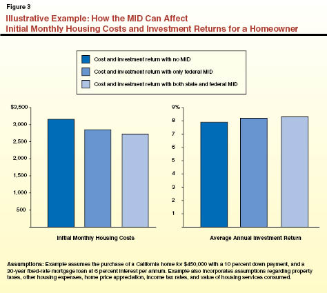
As noted above, the MID reduces the cost of housing by lowering the taxable income of homeowners based on the amount of mortgage interest they pay. Figure 3 provides an illustrative example of the impact of the federal and state MID on the monthly costs in the first year of ownership and the average annual investment return of a California home purchase under one common set of conditions. The example shows the initial monthly housing costs for a family of four having an adjusted gross income of $80,000 that purchases a $450,000 house. It also assumes a 10 percent down payment and a 30–year fixed–rate mortgage at 6 percent interest annually. As shown:

• The federal MID by itself reduces the monthly costs of housing in the first year by about $300 (roughly 10 percent) relative to what they would be without the deduction, and the state MID reduces these costs of another roughly $130 (about 4 percent).
The federal MID increases the rate of return on this housing investment by about three–tenths of 1 percent, and the state deduction further raises it by about another one–tenth of 1 percent.

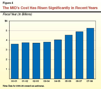
Revenue Impact of the MID

We estimate that in 2006–07, California taxpayers used the MID to reduce their income tax liabilities by $4.9 billion. As can be seen in Figure 4, the value of the MID has increased substantially in recent years. For example, the MID cost $3.6 billion in 2000–01. As shown in Figure 5, the MID is now the largest tax expenditure in California.

 

Figure 5 The MID Is California’s Largest TEP
(In Millions)
Top 12 TEP Programs	Type of Provision	2006-07 Revenue Reduction
Mortgage interest expenses	PIT deduction	$4,885
Food products	SUT exemption	4,748
Employer contributions to pension plans	PIT exclusion	4,450
Employer contributions to accident and health plans	PIT exclusion	3,975
Basis step-up on inherited property	PIT exclusion	3,030
Gas, electricity, and water	SUT exemption	2,468
Prescription medicines	SUT exemption	1,926
Capital gains on sales of principal residences	PIT exclusion	1,770
Dependent exemption	PIT credit	1,650
Charitable contributions	PIT deduction	1,600
Subchapter S corporations	CT special filing status	1,500
Real property taxes	PIT deduction	1,315
Note: Amounts shown for SUT exemptions include both state and local revenue reductions.
MID=mortgage interest deduction; TEP=tax expenditure program; PIT=personal income tax; SUT=sales and use tax; and CT=corporation tax.

Who Benefits From the MID?

Figures 6 and 7 show how many California taxpayers claim the MID and the amount of tax savings at each income level. The benefits of the MID are strongly skewed toward higher–income taxpayers. As discussed below, this is because higher income households both purchase more housing and are taxed at higher marginal income tax rates (which causes the MID’s benefit for each dollar of interest paid to rise with income).

Figure 6 How the MID’s Benefits Are Distributed by Income Group
(2004 Income Year)
	Taxpayers Benefiting			Tax Reduction
	Number (In Thousands)	Share of Total		Amount (In Millions)	Share of Total	Average Tax Reduction
Income Quintile
Bottom	8	0.2%		$1	—a	$108
Second	117	3.0		15	0.4%	128
Third	442	11.2		132	3.5	298
Fourth	1,281	32.6		743	19.6	582
Top	2,080	52.9		2,907	76.5	1,398
Totals	3,930	100.0%		$3,798	100.0%	$968
Breakout Within Top Quintile
Top 10 percent	1,091	27.8%		$1,868	49.2%	$1,713
Top 5 percent	535	13.6		1,049	27.6	1,960
Top 1 percent	93	2.4		201	5.3	2,158
a  Less than one-tenth of 1 percent.
Detail may not total due to rounding.
MID = mortgage interest deduction.

 

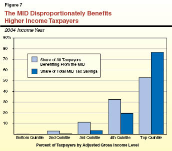
In particular, the figures show that in 2004 (the latest year for which detailed data are currently available):

• 3.9 million Californians were able to reduce their tax liability via the MID.
• In the bottom three income quintiles combined (that is, the lowest income 60 percent of taxpayers), only 570,000 taxpayers—about 1 out of every 14 taxpayers in these groups—used the MID to reduce their tax liability. In the top income quintile, by contrast, more than 2 million taxpayers used the MID to reduce their tax liability, more than three–fourths of the taxpayers in this group.
• Almost one–half of the tax reductions from the MID went to the top 10 percent of the income distribution (taxpayers making more than $113,900 in 2004).
The average per taxpayer savings for taxpayers who received some tax benefit from the MID was $108 in the bottom quintile, $298 in the middle quintile, and $1,960 for taxpayers in the top 5 percent.

To What Extent Does the MID Actually Promote Homeownership?

As noted above, the MID both reduces the cost of owner–occupied housing and increases its rate of return as an investment. This has the effect of increasing the demand for homeownership. This increase in demand can have several different effects. First, it may lead to an increase in the price of housing. Second, it may result in more units of housing being constructed and sold. Third, it may lead to an increase in average home size and/or quality. The exact mix among these three effects is influenced by such factors as the nature of the demand and supply for housing, as well as taxpayers’ demand for goods other than housing. The precise split of increased expenditures between greater homeownership and the acquisition of larger and more expensive homes or other goods is difficult to isolate, however. This is partly because the effects of changes in the cost of homeownership can vary considerably both over time as well as among different geographic regions or localities within regions.

There is much evidence, though, that suggests the MID does not have a substantial impact on homeownership rates per se. One piece of evidence comes from comparisons across states. Connecticut, Illinois, Indiana, Massachusetts, Michigan, New Jersey, Ohio, Pennsylvania, and West Virginia all have a PIT, but do not allow for a MID. The homeownership rate in these states, however, is higher than the national average—just the opposite of what one would expect if the deduction were an effective incentive for homeownership. Similarly, there seems to be little difference in the homeownership rates between countries that allow a MID and those that do not (such as Australia, Canada, France, Germany, Israel, Japan, and New Zealand).

Additional evidence suggesting that the MID is ineffective at increasing homeownership comes from studies of the U.S. over time. The value of the MID varies depending on a number of factors such as inflation, marginal tax rates, and rules concerning other itemized deductions. These factors have changed substantially over the last 40 years. Homeownership rates, however, have not responded much to these changes.

What Explains This Limited Effect? It is not surprising that the MID appears ineffective at significantly stimulating increases in homeownership rates when one looks at the design of the deduction. This is because the deduction is much more valuable for people who are relatively well off or likely to be established homeowners purchasing a larger house, than for first–time homebuyers purchasing a starter house who often have more limited incomes. This is demonstrated in Figure 8, which shows as an illustration how the MID’s benefits (in both dollar terms and as a percent of mortgage costs) differ for four hypothetical households having very different income and housing situations. One example of the varying effects of the MID on different taxpayers is that the state tax savings for the household in Case C is almost 300 times as large as for the household in Case A.

Figure 8 Comparisons of How Much the MID’s First-Year Savings Can Vary for Different Types of Taxpayers
Taxpayers	Amount	Percent of Mortgage Costs
Case A—$45,000 Income and $200,000 Home Price
Federal MID benefits	$562	4.3%
State MID benefits	16	0.1
Case B—$75,000 Income and $350,000 Home Price
Federal MID benefits	$2,370	10.5%
State MID benefits	1,062	4.7
Case C—$150,000 Income and $750,000 Home Price
Federal MID benefits	$13,012	25.4%
State MID benefits	4,536	8.9
Case D—$800,000 Income and $3,000,000 Home Price
Federal MID benefits	$34,185	16.7%
State MID benefits	7,267	3.5
Note: Calculations assume 10 percent down payment; 30-year fixed-rate mortgage at 6 percent for conforming loans or 6.5 percent for jumbo loans; no closing costs; 2006 tax brackets; charitable deductions equal 2 percent of income; and joint-return taxpayer with two dependent children and other standard assumptions.

 

Figure 9 provides actual California tax–return data that further explains why the structure of the current MID tends to promote the purchase of larger and more expensive homes rather than basic homeownership (especially for first–time homebuyers). These data show that:

• One of the key reasons that the benefits from the MID accrue primarily to high–income taxpayers is that they are much more likely than low–income taxpayers to itemize their deductions. As shown in Figure 9, almost 85 percent of taxpayers in the top income quintile itemize, compared to less than 18 percent of taxpayers in the bottom two quintiles.
The second key reason why the benefits from the MID accrue primarily to high–income taxpayers is that these taxpayers receive larger tax benefits than do low–income taxpayers for the same–sized deduction. This is because of their different marginal PIT rates. The average marginal tax rate for MID claimants is 0.06 percent in the bottom quintile and 8.15 percent in the top quintile. Thus, for each $1,000 of interest deducted, the bottom–quintile taxpayers will reduce their taxes by 60 cents, while the top–quintile taxpayers will reduce their taxes by $82.

There are several reasons why marginal tax rates are lower for taxpayers in the lower–income quintiles. The first is that statutory tax rates are lower for low–income taxpayers. Another reason is that low–income taxpayers generally have smaller amounts of other itemized deductions to reduce their taxable incomes than do high–income taxpayers. For low–income taxpayers, therefore, much of the MID may simply replace the standard deduction they might otherwise have claimed, whereas for high–income taxpayers it is more likely that all of the MID will be in addition to other deductions already being claimed. Also, many low–income taxpayers would owe only a small amount of tax without the MID. These taxpayers receive no benefit from any portion of their MID above the amount that is needed to eliminate their tax liability altogether.

The result of the combination of high–income taxpayers being more likely to itemize and also receiving greater proportional benefits when they do itemize is that most of the benefits of the MID are going to the taxpayers who would own a home absent the tax incentives.

Policy Options for Improving the State’s MID

The discussion above suggests that a case can be made for not having a state MID. This is primarily because the deduction is an ineffective means of increasing homeownership. In addition, from the state’s perspective, any benefits of attaining the goal of more homeownership are achieved by the federal MID. Any additional impact of the state’s MID is likely minimal. If the state MID were to be eliminated on a revenue neutral basis, PIT tax rates could be lowered—on average, by roughly 10 percent. Such tax rate reductions could be used to provide general tax relief or to provide each income bracket with relief comparable to the value of the MID that it could no longer claim.

If, however, the Legislature prefers to maintain a state–level tax incentive to promote homeownership, we believe the state should focus subsidies on those taxpayers who are less likely to own a home without tax incentives. A number of different options exist for making state housing tax policy more effective and cost–efficient. These options are listed in Figure 10. The next section describes possible modifications to the MID that would better target the associated tax savings to taxpayers whose homeownership behavior may be affected by them. The section after that recommends a more substantial change to California’s tax policy approach with respect to housing—replacing the MID with a tax credit.

Figure 10 Options for Modifying California’s MID

Modify the Current MID

Restrict the MID to interest paid on a single principal residence, thereby eliminating eligibility of second homes.

Eliminate the current MID for home equity loans.

Reduce the current $1 million cap on the size of a mortgage loan for which interest can be deducted.

Apply a means test under which the allowable deduction for mortgage interest phases out as income rises.

Restrict the MID to first-time homebuyers.

Restrict the MID to a limited number of years once a home is purchased and a mortgage loan is taken out.

Make the MID an “above the line” deduction available even to taxpayers who do not itemize their deductions.

Replace the MID With a Credit

Replace the current deduction with a nonrefundable credit.

Permit carry forwards into future years of mortgage credits not usable in a given year.

Replace the current deduction with a refundable credit.

Offer a flat dollar credit for homeownership.

Base the tax benefit not on the size of the mortgage loan but rather on some other criteria.

MID = mortgage interest deduction.

 

Options for Modifying the MID

Allow the MID Only for Principal Residences. The MID could be eliminated for purchases of second homes. Taxpayers who own their primary residence—the main policy priority—clearly would do so even if the purchase of a second home were not subsidized.

Eliminate the MID for Home Equity Loans. Taxpayers claiming deductions for equity loans already own their homes, so they would be very likely to continue owning a home even without this tax break.

Reduce the MID Loan Cap. Presently, the MID can be claimed on payments of interest on loans of up to $1 million. Most first–time homeowners, however, take out loans substantially smaller than this limit. Reducing the limit would, therefore, be much more likely to affect decisions about how big or expensive a home to buy rather than decisions about whether or not to own a home at all.

Means Test the MID. The MID could be phased out as taxpayers’ incomes rise. This, again, would probably not significantly affect the decision to own a home. As with all tax benefit phase–outs, however, this approach would increase tax complexity for many Californians.

Restrict the MID to First–Time Homebuyers. While this change might dissuade some people who already own houses from moving to larger houses, it is unlikely to induce people who already own a house to stop owning one.

Limit the Number of Years That the MID Can Be Claimed. A close variant of the preceding approach would be to allow the MID, but only for up to a specific number of years regardless of whether or not it was the taxpayer’s first home. This approach would still primarily target relatively new homeowners, but it would not penalize taxpayers who relocate soon after their first purchase.

Make the Deduction “Above the Line.” The MID could be made an “above the line” deduction, meaning that it would be available even to taxpayers who claim the standard deduction (and who generally have lower incomes), not just those taxpayers who itemize. This is the only option on this list that would increase the size of the MID tax expenditure’s cost.

Replace the MID With a Tax Credit

Alternatively, the Legislature could consider a more significant change in the way it subsidizes homeownership—by replacing the MID with a mortgage tax credit. Instead of allowing a deduction for the amount of mortgage interest paid, the state could offer a credit equal to a specified percentage of the amount of mortgage interest paid. If the MID were replaced with a credit, the value of the tax subsidy per dollar spent on a mortgage would no longer be dependent on one’s marginal PIT rate. This change would increase the homebuying tax incentive for taxpayers in low tax brackets relative to the tax incentive for taxpayers in high tax brackets, thereby focusing the tax benefits on the population whose decision whether or not to own a home is most likely to be influenced by the tax policy.

There are several different ways in which a tax credit could be allowed to offset taxes:

Nonrefundable Credits. With a nonrefundable credit, the dollar amount of the benefit a taxpayer may receive cannot be more than the tax they would otherwise owe. Thus, some taxpayers claiming the credit would not receive their full credit amount, especially if they had lower incomes and, thus, lower tax liabilities. Even a nonrefundable credit, however, would produce substantial shifts in benefits across taxpayers. For the families described in Figure 8, for example, the benefit of a state tax credit for family C would only be about twice as large as the benefit for family B, compared to more than four times as large for the MID.

Because subsidies to higher–income taxpayers would be reduced, the total budgetary cost of a credit would likely be less than for the MID, despite increasing benefits for some taxpayers. For example, if the state replaced the MID with a 5 percent credit on mortgage interest, more than one million Californians would have their tax bills lowered, yet the total cost of the program would drop by over $1 billion. The associated tax savings could then be used for whatever state policymakers felt was the highest priority, whether this be to reduce overall tax rates (benefiting everyone), to further increase the value of the credit to those who need it most, or for some other alternative.

Refundable Credits. Another option would be to issue tax refunds to taxpayers whose mortgage credits were larger than the tax they would owe without the credits. Such an approach would primarily benefit lower–income taxpayers and may, therefore, be an effective tool for increasing homeownership rates.

Tax administrators are often wary of refundable tax credits. This is because of both the processing activities involved and a concern that refundable credits necessitate significant enforcement activities to deal with fraudulent claims (based in part on prior experience with such refundable programs as the earned income tax credit). In this case, however, fraudulent claims might not necessarily be a major problem because the issuance of refunds could be made contingent on verification of eligibility via third–party information reports (primarily Internal Revenue Service Form 1098, which reports on mortgage interest payments).

Nonrefundable Credits With Carry Forwards Allowed. When policymakers want to help taxpayers who do not have any tax against which to apply their tax credits, but do not want to allow credits to be refundable, they often allow the credits to be carried forward for use in future tax years. This approach would provide some benefit to households who have low incomes at the time of their home purchase but are able to increase their income in later years. Of course, this benefit would not be as valuable as receiving a tax refund in the early years when their income is low, and this approach would provide no benefits for taxpayers whose income never rises to taxable levels.

In addition to deciding about the type of credit, the Lesislature would also face choices about the structure of the credit.

Limiting the Amount of Interest That Can Generate a Credit. Any of the policy options described above that could be used to limit the scope of the MID could also be applied to a mortgage tax credit. Thus, interest paid on mortgages for second homes or on home equity loans could be ineligible for the credit. The current cap under which only interest paid on the first $1 million borrowed is deductible could be retained or lowered with a credit. A credit could also be means tested, restricted to first–time homebuyers, or claimed for only a limited number of years.

Basing the Credit on Something Other than Interest Payments. Another policy option that could be considered is basing the size of the credit on something other than the size of the taxpayer’s mortgage. For example, the state could provide a flat dollar credit amount to all homebuyers. The housing tax credit could be set equal to a specific amount, such as $1,000 per year. If a flat credit were adopted, there would be no tax incentive for buyers to buy larger homes rather than smaller ones, and the greatest tax benefit relative to the purchase price would go to those taxpayers struggling to afford any house at all.

Reforming the MID at the Federal Level

Economists and policymakers have considered many of the same policy options discussed above for modifying the federal MID. For example, in its recent review of the budget–balancing options, the Congressional Budget Office identified as options and analyzed the effects of (1) lowering the cap for the MID from interest on mortgage loans of $1 million to interest on mortgage loans of $400,000, and (2) replacing the MID with a 15 percent credit on mortgage interest paid. Similarly, in 2005, the President’s Advisory Panel on Tax Reform recommended replacing the MID with a tax credit equal to 15 percent of mortgage interest paid, limited to the amount of interest paid on the average regional price of the housing involved.

Practical Considerations—Transitioning to a Credit

The most difficult aspect of many tax policy changes involves their initial implementation. If the state were to change from the current MID to a credit, the biggest transition issue would be how to treat taxpayers who only recently purchased their homes. To many people, it would seem unfair to change the tax benefits associated with existing mortgages after homes have already been purchased and financial commitments made.

One Possible Solution—Grandfathering

The above problem can be dealt with by “grandfathering in” the current deduction for existing mortgages. With grandfathering, the tax value of existing mortgages would be unchanged. There are disadvantages to this approach, however. One is the administrative burden arising from having to track and record two different methods of treating home acquisitions. In addition, there would be those who feel it is unfair that some people will continue to enjoy greater benefits than others.

This problem would diminish over time as, each year, there would be fewer grandfathered mortgages remaining. However, it would persist as long as old mortgages are still outstanding. At some point, the administrative burden from maintaining dual systems for both old and new mortgages might become large relative to the perceived unfairness in changing the tax treatment of taxpayers still paying off old mortgages. It might make sense, therefore, to establish a cutoff date—say, 15 years after enactment of a change to a credit—after which the new rules would apply to everyone and deductions would no longer be available.

Another Approach—Phasing–In a Change

Another approach to the transition that has been suggested by some economists is to ratchet down over time the limit on the interest deduction. For example, the deduction could be limited to the interest paid on $800,000 of mortgage debt the year after enactment, interest paid on $600,000 of debt the following year, and so forth. This approach would compress the time needed for the transition to the new tax system. It would, however, place an administrative and recordkeeping burden on both the state and on affected taxpayers. It would also reduce the tax benefits of many existing mortgages.

Economic Effects

The proposed change from a deduction to a credit for homebuyers would benefit some taxpayers and hurt others. It would also have a variety of impacts on the housing sector, consumer spending, and other segments of the economy.

Higher–Income Taxpayers

Those taxpayers in the highest income brackets would receive smaller tax subsidies for their mortgage borrowing. Many of these taxpayers would respond by borrowing less money. For some of these taxpayers, this change would merely represent a portfolio shift. In other words, they would sell some of their other assets to increase their housing–related down payments and do less mortgage borrowing, but still purchase the same house they would have anyway.

Other high–income taxpayers, however, would respond to the decrease in the tax subsidy for borrowing by reducing the amount that they are willing to spend to purchase houses. As a result, there would be some decline in housing prices at the high end of the market.

To the extent that housing prices dropped, the burden of the reduced value of the tax incentive for home purchases would be shifted from purchasers of houses to people who own homes at the time of the change in tax law. People buying homes would realize losses from the reduced value of the tax break but gains from the price reduction on homes. On the other hand, people who own homes at the time of the law change would be hurt by the reduction in housing prices.

Lower–Income Taxpayers

At the low end of the housing market, prices are not likely to drop, and could even be boosted. This is because many lower–income taxpayers would receive a larger tax benefit under the proposed credit than under the current MID. Therefore, demand for relatively inexpensive housing, and, hence, housing prices should not face much downward pressure in this segment of the market.

In the long run, we would expect home builders to respond to the new tax regime by building relatively more houses for the less expensive segment of the market where demand would be stimulated, and relatively fewer in the expensive segment where demand would decrease. This adjustment would be necessary to restore equilibrium to the housing market.

Summary and Conclusions

Both the federal and California tax codes contain a variety of provisions that subsidize housing purchases. Tax policy generally strives to avoid favoring certain sectors of the economy over others, unless there are persuasive reasons for doing so. Housing does appear to be one sector of the economy for which some preferential treatment may be appropriate. In particular, some level of housing subsidy can be justified on the grounds that, because homeownership appears to provide benefits to society in general, the free market by itself may not produce optimal levels of homeownership.

The largest explicit state housing subsidy is the MID. It is poorly designed, however, for achieving the policy goal of increasing the rate of homeownership. The structure of the MID directs most of its benefits to taxpayers who would own a home even if the MID did not exist, rather than to those whose rent–or–own decision may be influenced by the presence of the MID. Its benefits are skewed toward higher–income taxpayers, and it encourages the purchase of large and expensive homes.

There are, however, a number of options for modifying the MID to more efficiently achieve the goal of increased homeownership rates. We believe it would be even more beneficial for the Legislature to replace the MID with a tax credit for home purchases.

Appendix

Background Relating to Housing’s Tax Treatment

What Would an Economically Neutral Tax Treatment Look Like?

A good place to begin in evaluating housing tax policy is to describe the tax treatment that would be appropriate if our only policy objective were economic neutrality. The appropriate tax treatment of housing is complicated by the fact that housing plays two distinct roles in the economy. One of housing’s roles is as a business investment that produces a flow of housing services over time. Its second role is as a consumption good whose residents are using housing services over time. Most economists would argue that the tax system should treat business investment in housing like other business investments, and should treat the consumption of housing like the consumption of other goods. That is, homeowners who live in their own houses would be treated both as (1) landlords renting their property (to themselves) and (2) consumers renting their property (from themselves). Under such an approach, the homeowner–landlord can then be treated just like any other landlord, while the occupants of owner–occupied homes can be treated like other consumer–occupants.

Tax Treatment as Landlords

Landlords must include rent received as income when calculating their income taxes. To put homeowners on an equal basis, we would need to attribute to them an amount of rent that would have been charged for each house were it occupied by someone other than its owner, and include that amount in the homeowner’s income for tax purposes. Landlords also must pay taxes on capital gains received when they sell properties. Thus, to be consistent, homeowners would not receive a capital gains exclusion for sales of their principle residences as they do currently. On the other hand, landlords get to deduct all relevant costs of owning and maintaining houses as a business expense. Therefore, under this approach, homeowners would be allowed to deduct from their taxable income all similar expenses that they incur, including mortgage interest, property taxes, depreciation, and home maintenance expenses.

Tax Treatment as Consumers

To be placed on equal footing with housing occupants who are not owners, homeowners would receive the same tax treatment as renters. California’s Homeowner’s and Renter’s Assistance Program follows this guideline for tax relief programs as long as it provides the same amount of assistance to homeowners as to renters with the same level of income. By comparison, the renter’s credit would be eliminated in this idealized, economically neutral tax system, because it subsidizes renters and not owners.

Should Government Try to Influence the Housing Market?

As noted in the text, many people believe that government should encourage homeownership by assisting people who wish to purchase houses. When discussing the programs that the government has adopted in this area and evaluating the MID in particular, it is important to also consider the case for government encouragement of homeownership itself.

According to economic theory, people will choose to purchase homes whenever doing so makes them better off, and choose to not purchase homes when purchasing them would make them worse off. This decision takes into account both what a person would like to do and, also, their ability to purchase a home. Thus, the decision to buy a home incorporates factors such as the purchaser’s income level, housing prices, the costs of other goods and services that they might value, and their preferences.

In some cases, policymakers choose to intervene in the marketplace and make all goods and services, including housing, more able to be purchased than otherwise for certain individuals and groups. This is most commonly done specifically to assist lower–income individuals. This type of nonspecific intervention is economically neutral with respect to the different types of goods and services consumed.

In other cases, however, the government adopts policies to encourage the purchase of specific types of goods and services, whether for all taxpayers or selected groups. This second approach is especially appropriate when the consumption of a good or service produces a greater value to society than just to the individuals most directly involved.

In the case of housing, this means that government intervention can be justified if society in general benefits from having more individuals own their own homes. There are many reasons to think that such societal benefits exist, such as the incentives homeownership gives the occupants to do a better job of maintaining their residences than landlords and their tenants might. Given such factors, we assume in this report that the state is pursuing a policy goal of increasing homeownership on the grounds that it produces socially valuable benefits.

Acknowledgments This report was prepared by David Vasché . The Legislative Analyst's Office (LAO) is a nonpartisan office which provides fiscal and policy information and advice to the Legislature.

LAO Publications To request publications call (916) 445-4656. This report and others, as well as an E-mail subscription service , are available on the LAO's Internet site at www.lao.ca.gov. The LAO is located at 925 L Street, Suite 1000, Sacramento, CA 95814.

---

Return to LAO Home Page